PE to ARCS Migration Reference

This document compares the functional differences between the PE and ARCS systems in three major aspects — project management, script interfaces, and system configuration — to help users migrate smoothly from PE to ARCS.

---

1 Project Management

1.1 New Project Feature Comparison

Feature	PE	ARCS
New project	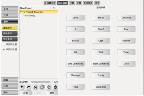Click New to create a new project; a root node (New Project) appears in the program list.	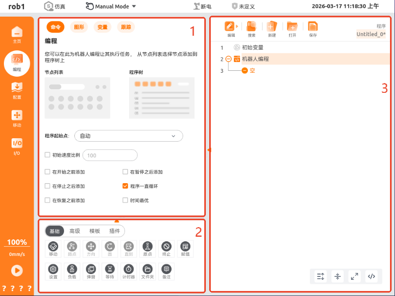You can create or write robot programs through the 【Programming】 interface. Click New to create a new project; a robot program appears in the program list.
Save project	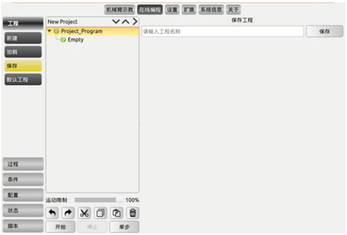Click the save button on the far left, enter a name, then click the save button on the right to save the project. Project files are saved in xml format.	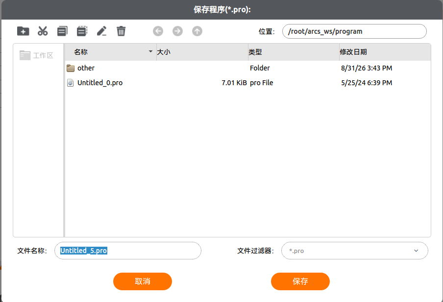Click the save button, enter a file name, then click the save button below to save the project. Project files are saved in pro format.
Default project	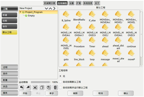Click Default Project, select the project to operate on from the default project file list, and check different options as needed. Check Auto-load default project to automatically load the default project after opening the programming environment. Check Auto-load and run default project to automatically load and run the default project after opening the programming environment. Click OK to confirm the default project configuration.	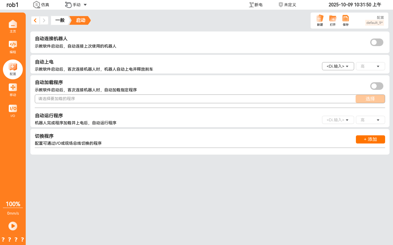Click 【Configuration】 and then the 【Startup】 tab in turn to configure the default program and auto initialization. The default program is the program automatically loaded after the controller powers on; when the system enters the program-running state without any loaded program, it automatically loads the default program. When Auto-connect robot, Auto power-on, and Auto-load program are enabled, the robot runs the program immediately after the controller is powered on, as long as the input signal matches the selected signal level. For example, at low level, no edge transition to the selected signal level is required. Be careful when the signal level is set to low level. The input signal defaults to low level, which causes the program to run automatically without being triggered by an external signal.
Load project	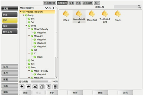Click Load, find the target program, and load the project. After opening, the opened program is loaded into the program list.	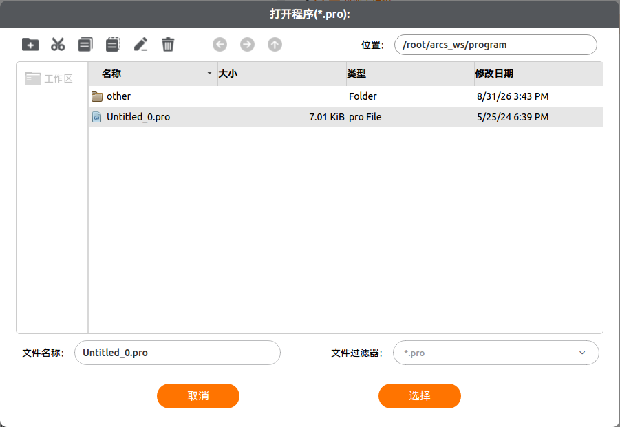Click Open, enter the password, find the target program, and load the project.
Run project	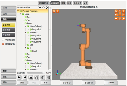After the project file is edited, you can click Start to run the project. The steps are as follows: • Click the Start button at the bottom of the interface; • Long-press Auto Move until the robot arm reaches the initial point (the cancel button shows OK); • Click the OK button; • Click the Start button again.	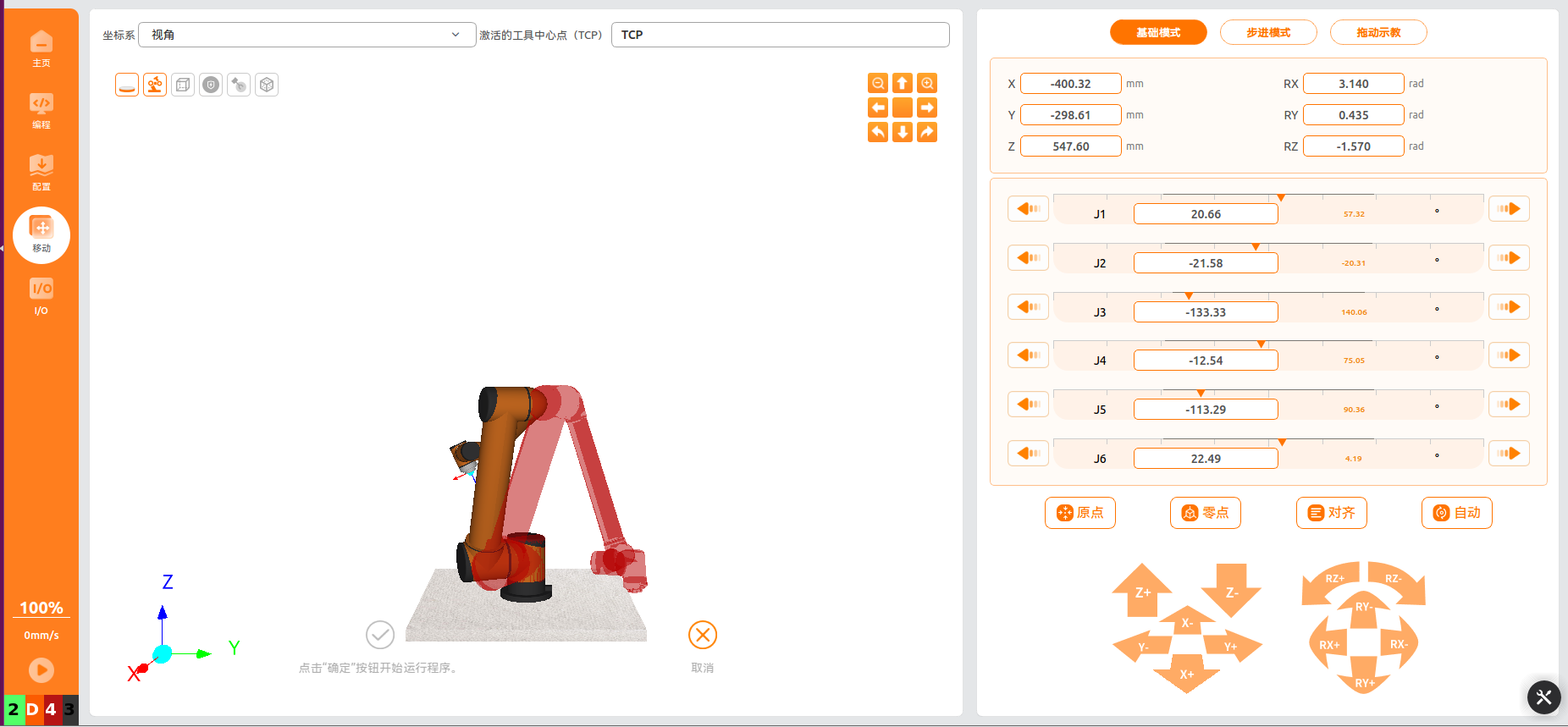Click the 【Run】 button in the left menu bar, select 【Run program from start point】, and enter the 【Move】 interface. Long-press 【Auto】 until the button turns gray to move the robot arm to the program's initial pose. Then click the 【Click OK to start program】 button to run the program.

1.2 Sub-project Feature Comparison

Feature	PE	ARCS
Create procedure file	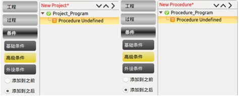Procedure is a sub-project (procedure) editing command. In a Procedure program block, you can edit reusable program segments and conveniently load them into other project program blocks. Sub-project commands can be called from both project files and sub-project files. Click New under Project or Procedure in the toolbar, and New Project or New Procedure is displayed in the project logic area.	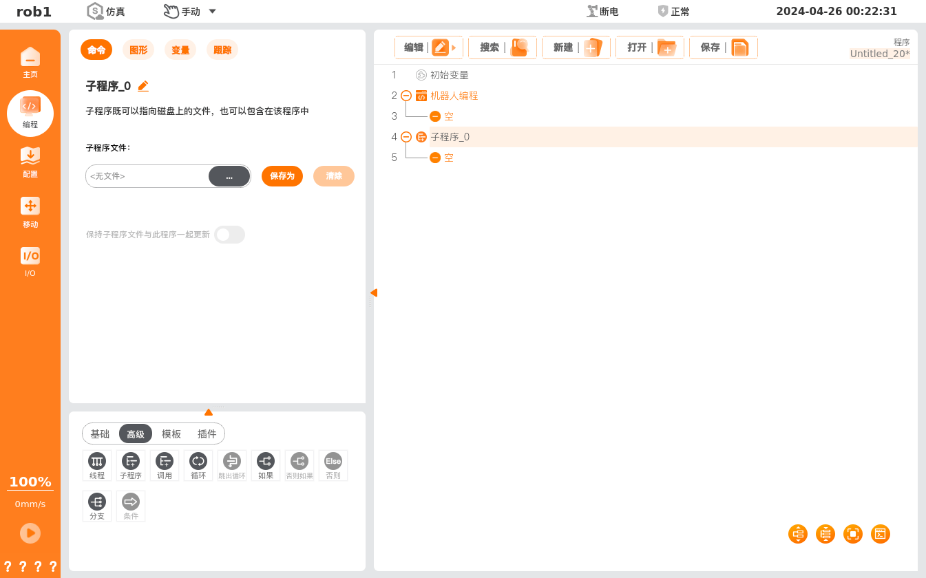…: Load a previously written program Save As: Save the subprogram as a separate file on disk. Clear: Clear the file opened in the subprogram. Keep the subprogram file updated with this program: when checked, modifications made in the opened subprogram are automatically saved to that subprogram file.
Call sub-project command	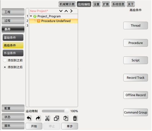Create a project or procedure file, select Advanced Conditions, and click the Procedure command. 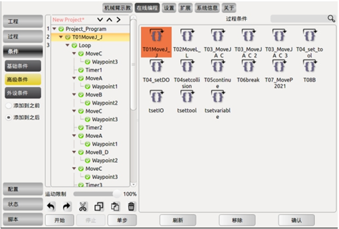Select Procedure Undefined in the project list, and the callable sub-project files are displayed in the properties window. Select a sub-project file and click OK to call it; the commands in the called sub-project file are then displayed in the project list. • Click Refresh as file update button to scan the current file save directory and update the display of file changes. • Click Remove to delete the selected Procedure.	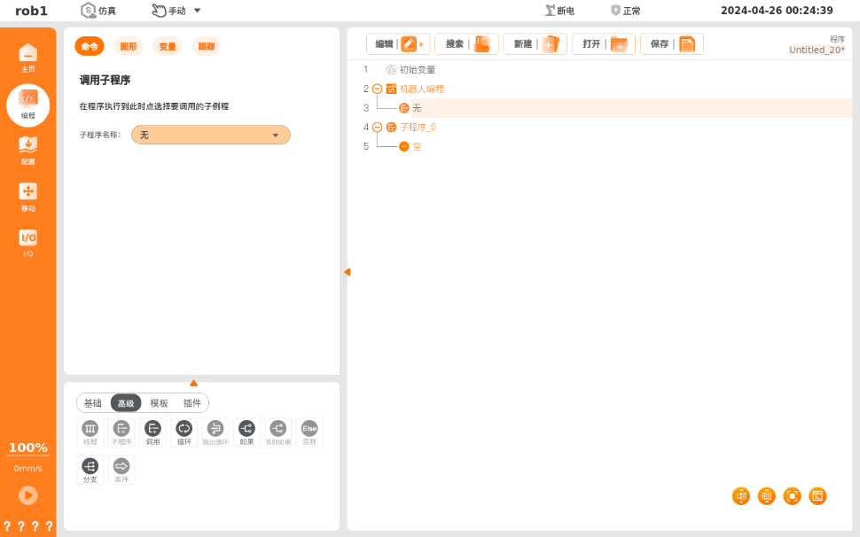The 【Call】 command calls a subprogram. When the program executes this node, it jumps to the called subprogram and runs it.

1.3 Move Command Feature Comparison

Feature	PE	ARCS
Add command	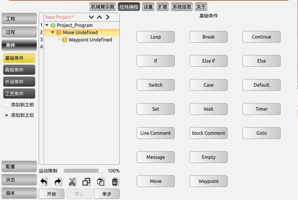The Move command is used for movement operations of the robot end tool center point between waypoints. The robot's motion is controlled through basic waypoints, and waypoints must be placed under motion commands. • Add a Move node to the program list; it contains a Waypoint node underneath. • Click the input box to the right of the nickname to modify the command name. • Select the Move node to configure the state of the Move command. • Click Remove to delete this Move command. • You must click OK to confirm the configuration is complete and save it.	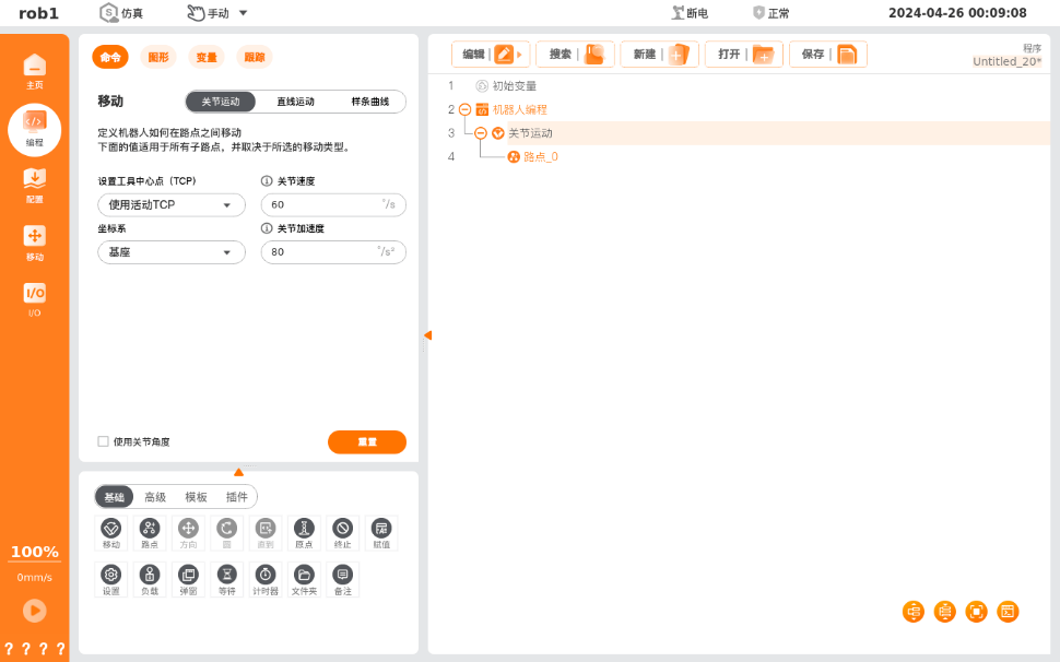Click the 【Move】 icon, and a 【Joint Motion】 node is added to the program tree, containing a 【Waypoint】 node underneath. The 【Move】 node contains move types: Joint Motion, Linear Motion, and Spline Curve. The display name of the 【Move】 node in the program tree is determined by the selected move type. Select the 【Joint Motion / Linear Motion / Spline Curve】 node to configure that node.
Joint motion	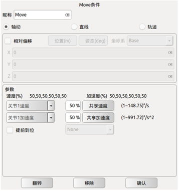Based on the running angles of each joint between waypoints and the limits of the configured maximum motor speed and maximum acceleration (common parameters of the six robot axes), all joints synchronously reach the target waypoint at the fastest speed (with zero start and end speeds). During joint motion, you can set the maximum joint angular velocity and maximum angular acceleration percentages for joints 1–6 individually; click the Share button to copy the speed or acceleration to other joints.	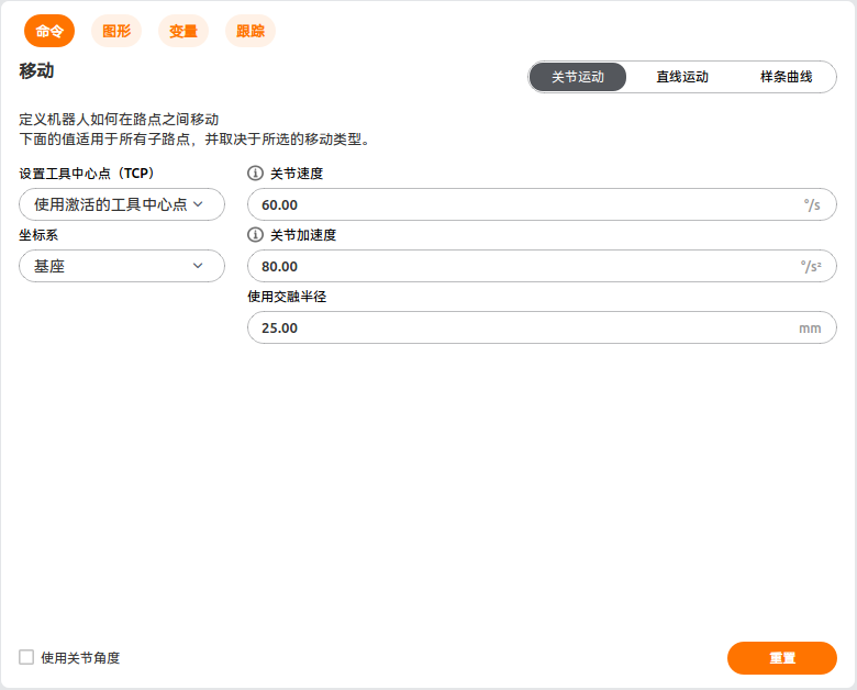Joint motion completes movement by controlling the robot joints. Joint motion provides a curved path for the tool center point (Tool Center Point, TCP). During motion, if blending parameters are set, the robot can smoothly transition between two trajectories, making its movement faster and more stable. Use joint angles: When checked, joint angles are recorded in the script during program execution, replacing the robot's position information. At the same time, the system disables 【Set Tool Center Point (TCP)】 and 【Coordinate System】 here. After enabling this feature, when a project is migrated, the robot will not adjust this waypoint information and the data remains usable.
Linear motion	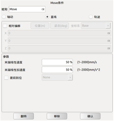Causes the tool center point to move linearly between waypoints. This means each joint performs a more complex movement to keep the tool on a straight-line path.	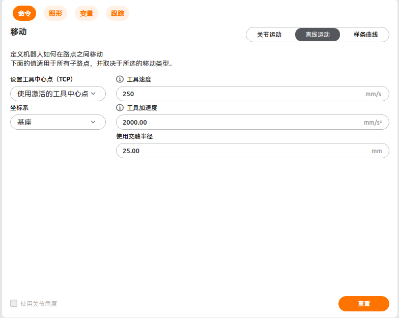Linear motion means the robot's tool center point (TCP) moves linearly to the target waypoint. This means each joint performs a more complex movement to keep the TCP on a straight-line path. Whether the tool speed can reach and maintain the maximum speed depends on the linear displacement and maximum acceleration parameters.
Arc and circle motion	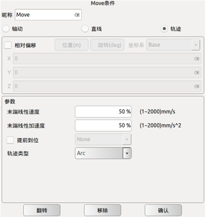The arc is determined by the three-point method, and motion proceeds in order from the start waypoint to the end waypoint; this belongs to Cartesian space trajectory planning. The orientation change is affected only by the start and end points. The meanings of maximum speed and acceleration are the same as for linear motion. When the trajectory type is set to Arc, it is arc motion. When the parameter type is set to Cir, it is circle motion, and the number of circle cycles can be entered in the text input box on the right.	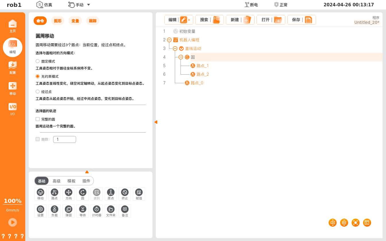The 【Circle】 command sets the TCP at the robot end to perform arc or circle motion at a constant speed. The arc or circle is determined by the three-point method, and motion proceeds in order from the start waypoint to the end waypoint; this belongs to Cartesian space trajectory planning. When the robot performs arc or circle motion, the start and end points affect the robot's orientation change, and the meanings of maximum speed and acceleration during motion are the same as for linear motion. Note: • The 【Circle】 node must be used under 【Linear Motion】. • The three points defining the circle must not be collinear; otherwise the system pops up an error. • The 【Circle】 node requires three waypoints: start point (Waypoint_0), via point (Waypoint_1), and end point (Waypoint_2). By default, all waypoints use the same blend radius. Direction mode: • Fixed mode: the tool orientation remains unchanged relative to the arc path coordinate system. • Unconstrained mode: the tool orientation changes linearly, rotating around a fixed axis in space, changing from the start-point orientation to the target-point orientation. • Via-point mode: the tool orientation starts from the start point, passes through the intermediate-point orientation, and changes to the target-point orientation. Select the circle trajectory: • Full circle: when checked, the robot performs a full circle motion following the circle determined by the three-point method. When unchecked, the robot moves along a circular trajectory between the start, via, and end points, and after reaching the end point it returns to the start point along a linear trajectory. • Number of turns: sets the number of turns for full-circle motion.
B-spline	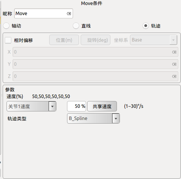B-spline curve (B_Spline): fits a path curve based on the given path points. The more waypoints used to generate the fitted curve, the closer the fitted curve is to the expectation. A B-spline curve is a smooth curve passing through all the given waypoints; note that the start and end points of the curve cannot be closed.	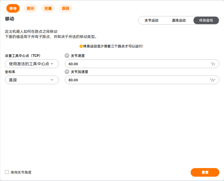A spline curve means the robot fits a curved path based on the given waypoints and passes smoothly through all the given waypoints at a constant speed. The more waypoints given on the expected curve, the better the fitted curved path matches the expectation. Configure the related parameters of this spline curve: TCP, coordinate system, joint speed, joint acceleration, etc. Add multiple 【Waypoint】 nodes under the 【Spline Curve】 node and set each waypoint's position to complete adding the 【Spline Curve】.
Waypoint command	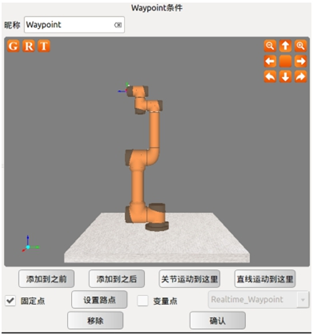Click the input box to the right of the nickname to modify the command name. After the nickname is changed, you can customize the waypoint's global function. When a waypoint with the same nickname is created, the data of the originally named waypoint takes precedence; for a waypoint whose nickname and related parameters have been modified, the modified waypoint nickname and parameters take precedence. • A Waypoint can only be added after a Move command. • Click Add Before to add a new waypoint before this waypoint. • Click Add After to add a new waypoint after this waypoint. • Click Move Here to move the robot to the current waypoint; this is effective for a real robot. • You can choose joint motion to here or linear motion to here. • Click Remove to delete this waypoint. • Click Set Waypoint to set the position and orientation of the waypoint. After clicking Set Waypoint, the panel automatically switches to robot arm teaching; the user can move the robot end to the new waypoint position and then click the OK button in the lower-right corner. • Click OK to save this waypoint's state configuration; a popup appears showing that the condition has been saved. Variable waypoint (variable point): Select Variable Point in the waypoint condition interface and confirm; this waypoint becomes the waypoint set in the variable settings. When the waypoint in the variable is changed, all waypoints in the project file change accordingly. This feature can batch-change the parameters of identical waypoints to save programming time. A variable point corresponds to a variable of type pose in the variable configuration. 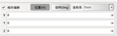Relative waypoint (relative offset): The user controls the motion of the robot arm or the end-tool coordinates through position or orientation offsets relative to the selected coordinate system.	The 【Waypoint】 command is the position point that the robot's tool center point (TCP) will reach; by setting waypoints you can set the specific positions of the robot's motion. Usually the motion trajectory of the robot's tool center point (TCP) is composed of two or more waypoints. The 【Waypoint】 node can be configured with three types: 【Fixed Position】, 【Variable Position】, and 【Relative Position】. 【Fixed Position】: Set the 【Waypoint】 pose by operating the robot's 【Move】 interface or dragging the robot. 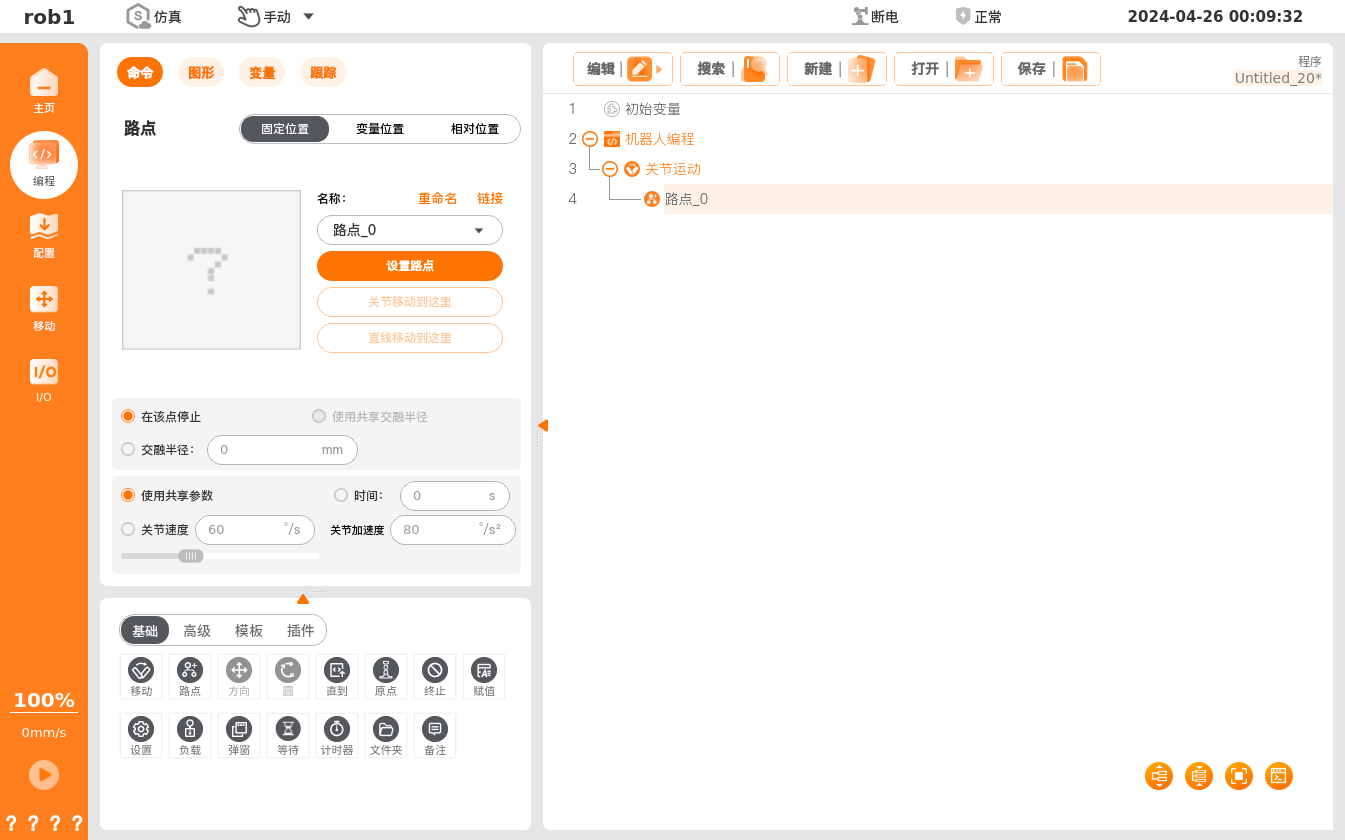In the 【Fixed Position】 interface, click 【Set Waypoint】 to switch to the robot teaching interface; you can use the 【Position/Orientation Control Buttons】 on the interface to move the robot, or enter drag-teaching mode to manually move the robot to the target waypoint. After setting, click the 【OK】 button to save the 【Waypoint】 pose. 【Waypoint】 naming and switching: The default waypoint name is "Waypoint_n", where n starts at 0 and increments by 1 for each new waypoint. Rename a waypoint: click 【Rename】 to modify the waypoint name, but duplicate waypoint names are not supported. Link: click the icon or click 【Link】 and select a waypoint in the program to use the target waypoint's pose. After a successful link, the 【Link】 button changes to 【Unlink】; click 【Unlink】 to restore the original waypoint. Blending parameters: • 【Stop at this point】: the blend radius is 0 mm, and the robot stops at this waypoint position. • Use shared blend radius: set this waypoint to use the shared blend radius (this option is unavailable for joint motion and spline curves). • Use blend radius: set this waypoint's blend radius. Speed: • Use shared parameters: set this waypoint to use the shared speed parameters (joint/tool speed, joint/tool acceleration). • Time: set the total movement time from the previous waypoint to this waypoint (unit: s); this setting affects the robot's speed. Setting an unreasonable total movement time may cause the robot's motion parameters to exceed the robot's parameter range; AuboStudio optimizes this, so the parameters at robot runtime prevail. • Joint/tool speed, joint/tool acceleration: set the joint/tool speed and joint/tool acceleration of this waypoint. 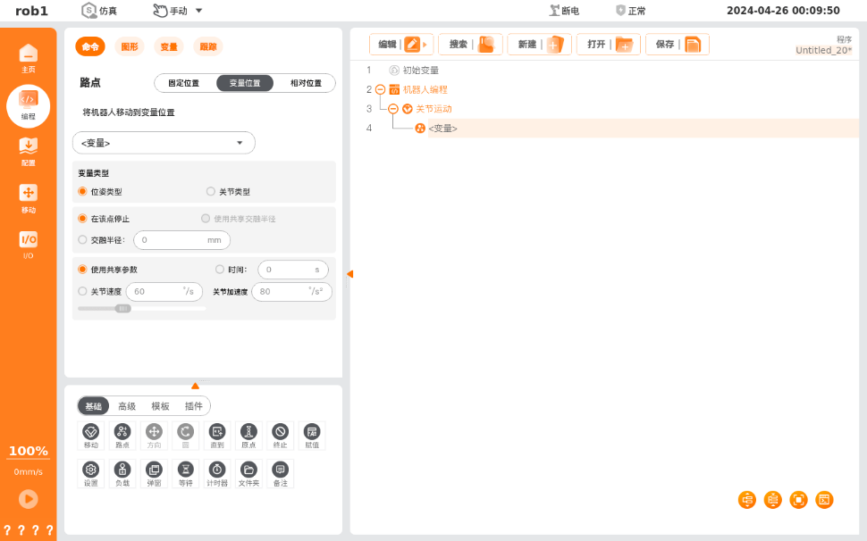【Variable Position】: Set the 【Waypoint】 pose by configuring variables. 【Variable Position】 is often used to batch-change the parameters of identical waypoints to save programming time. Select variable: click the 【<Variable>】 drop-down box and select a variable. For variable settings, see Assignment and Variables. Variable type: set the type of the variable. • Joint type: the six parameters of the variable correspond to the six joint angles, in radians (rad). For example: i_variable_1 = {0, -0.261796, 1.74532, 0.436316, 1.5708, 0}. • Pose type: the six parameters of the variable represent the Cartesian pose of the robot end, in the format {x, y, z, roll, pitch, yaw}: the first 3 parameters x, y, z are the position coordinates of the end in the world coordinate system, in meters (m); the last 3 parameters are the end orientation angles (Roll, Pitch, Yaw, i.e., the RPY Euler angle representation), in radians (rad). 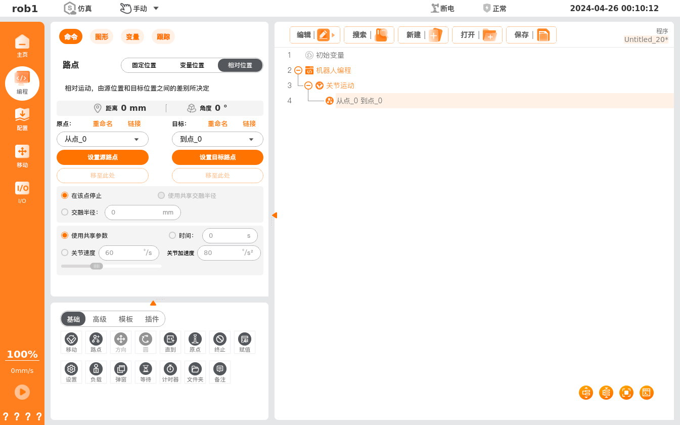【Relative Position】: Defines the 【Waypoint】 pose through the difference between two given positions (source waypoint and target waypoint). Note: when programming, the program must contain at least one waypoint other than the 【Relative Position】 waypoint; otherwise unpredictable errors may occur in the robot. • Distance: the Cartesian distance between the source waypoint and the target waypoint. • Angle: the length of the rotation vector of the direction change between the source waypoint and the target waypoint. • Set source waypoint, Set target waypoint: after clicking, switch to the robot teaching interface and use the 【Position/Orientation Control Buttons】 on the interface to move the robot, or use teaching mode to manually move the robot to the target waypoint. After setting, click the 【OK】 button to save the pose of the source or target waypoint.

1.4 Basic Condition Command Feature Comparison

Feature	PE	ARCS
Loop command	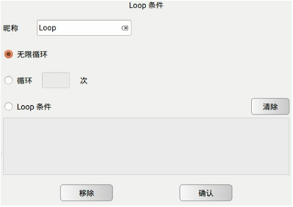The Loop command can be used to repeat program code multiple times in succession. Program code that needs to be repeated is placed in the loop command. The loop command can be configured to repeat infinitely, a specific number of times, or while an expression is true (for example, a variable or input signal). • Loop is a loop command; the programs contained in the Loop node run cyclically until the termination condition is met. • Click the blank field to the right of the nickname to pop up an input box and modify the command name. • Select Infinite Loop to run the program in an infinite loop. • Select Loop __ times to set the number of loops; the loop exits after reaching the count. • Select Loop condition to set the loop condition expression; enter the loop when the expression is true and exit when it is false. Click Clear to clear the expression. • Click OK to confirm this command's state configuration and save it.	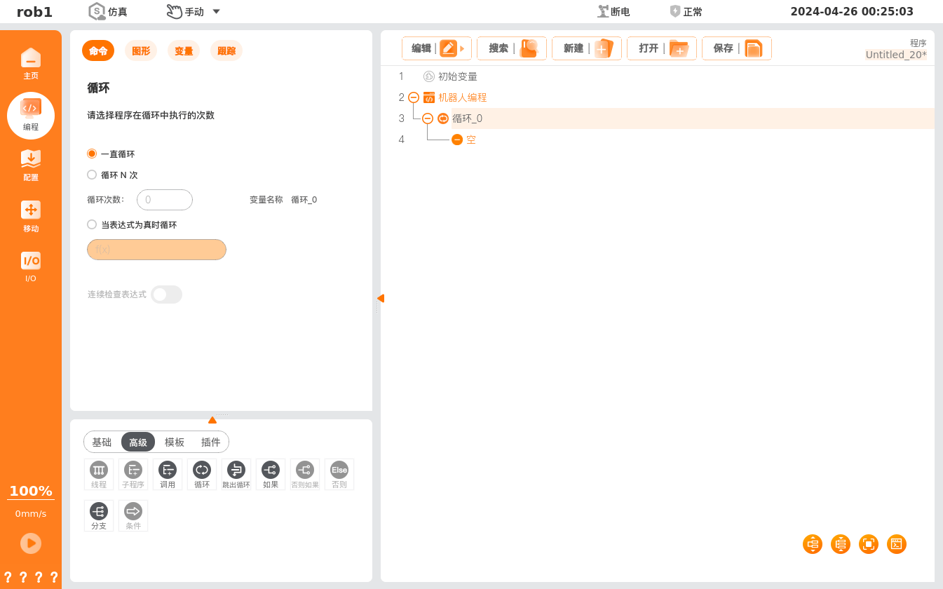The 【Loop】 command creates a loop program block. • Loop forever: when checked, the nodes in the program block run in an infinite loop. • Loop N times: when checked, set the "loop count"; N is the number of loops, and the nodes in the program block run N times. The program creates a dedicated loop variable (e.g., loop_0 shown in the figure), which can be used in expressions inside the loop. After entering the loop, the loop variable counts from 0 to N-1, and the loop ends. • Loop while the expression is true: when checked, set the expression. When the program reaches this node, it first checks whether the expression is true: if true, it enters the loop and runs the nodes in the program block; if false, it skips this loop. • Continuously check expression: when checked, the expression is checked continuously while the loop program block is executing; as soon as the expression is false, it exits the 【Loop】 program block at any time.
Break command	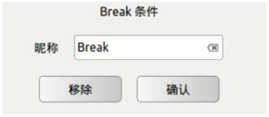The Break command exits a loop; when the Break condition is met, the loop is exited. • Click the blank field to the right of the nickname to pop up an input box and modify the command name. • Note the syntax when using the Break command: Break can only be used inside a Loop, and there must be an If command before the Break. When the condition in the If is true, the Break command runs and exits the loop; otherwise an error is displayed. • Click Remove to delete this Break command.	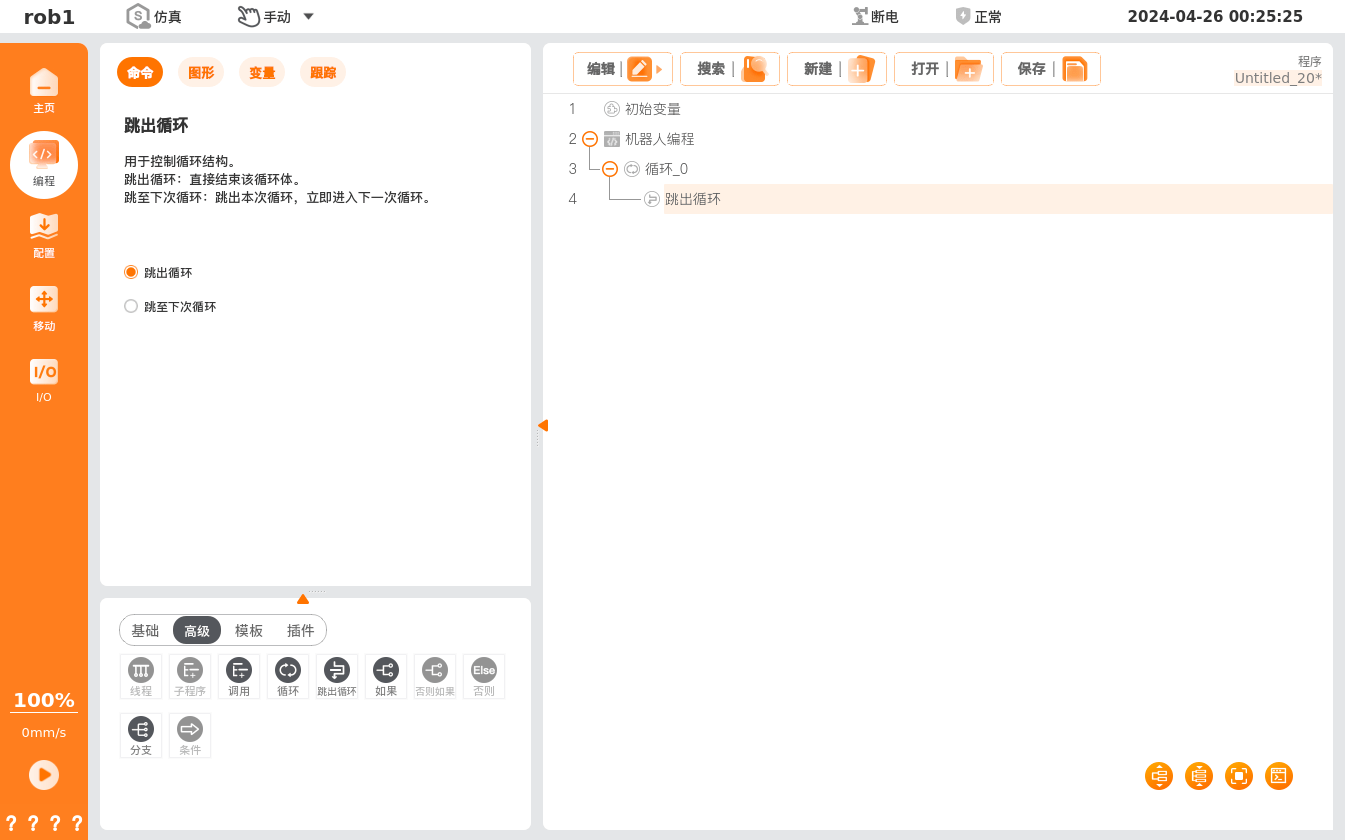Set the exit mode: Break the loop: directly exit the loop and run the next program node after the loop node.
Continue command	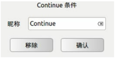Continue ends a single loop iteration; when the Continue condition is met, the current loop iteration ends. Note the difference from the Break command: Break exits the entire loop and does not re-enter, while Continue exits a single iteration and the loop is re-entered in the next cycle.	Set the exit mode: Skip to the next loop. Exit the current iteration and immediately enter the next iteration. If the loop node does not require variable or expression evaluation, it directly enters the next iteration. If the loop node requires variable or expression evaluation, the evaluation is performed first: if true, enter the next iteration; if false, end the loop.
If command	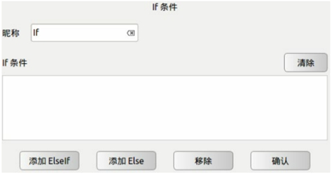If…else is a conditional selection command that runs different program branches based on the condition. • Click the blank field to the right of the nickname to pop up an input box and modify the command name. • Click the blank window under the If condition to pop up an input box where you can enter the conditional expression; the expression follows C language operator rules. When the expression is true, the programs contained in the If node execute; if false, the programs in the Else or Else if node execute. • Click Remove to clear the expression. • Click Add Else if to add an Else If node. One If can add multiple Else If nodes. • Click Add Else to add an Else node, forming an If…Else combination with the current If node. One If can add only one Else. • Click Remove to delete this If command; the Else If and Else corresponding to this If are also deleted. • Click OK to confirm the state configuration and save it.	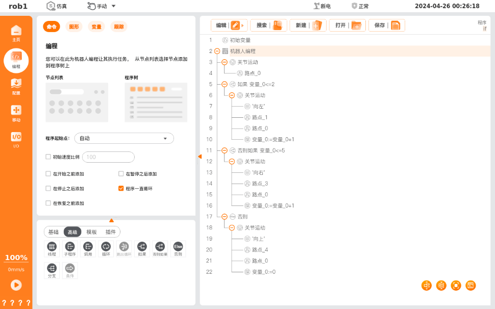The 【If】 command creates a conditional program block. The 【Else If】 command creates a conditional program block under the If node. The 【Else】 command creates a program block under the If or Else If node. If settings: Click the expression on the If interface to edit the conditional expression. Continuously check expression: when checked, the conditional expression is checked continuously while the If program block is executing; as soon as the conditional expression is false, it exits the If program block at any time. Else If settings: Click the expression on the Else If interface to edit the conditional expression. Continuously check expression: when checked, the conditional expression is checked continuously while the Else If program block is executing; as soon as the conditional expression is false, it exits the Else If program block at any time.
Conditional selection command	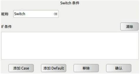Switch...Case...Default is a conditional selection command that runs different Case program branches based on the condition. It can be used to control the program flow according to the value of a variable. • Click the blank field to the right of the nickname to pop up an input box and modify the command name. • Click the blank window under the condition to pop up an input box where you can enter the conditional expression; the expression follows Lua language operator rules. When the Switch command runs, the program computes the value of the expression and compares it in order with the condition values of the Case statements below; if equal, it executes the program block under that Case; if no Case value satisfies the condition, it executes the program block corresponding to Default. • Note: true/false must be used for truth evaluation; 1/0 cannot be used as a substitute. • Click Remove to clear the expression. • Click Add Case to add a Case node, forming a Switch...Case combination with the current Switch node. One Switch can add multiple Case nodes. • Click Add Default to add a Default node. One Switch can add only one Default. • Click Remove to delete the selected Switch; the Case and Default corresponding to this Switch are also deleted. • Click OK to confirm the state configuration and save it.	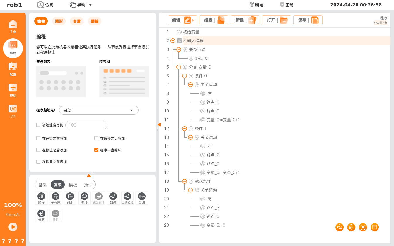Branch / Condition / Default The 【Branch】 command creates multiple branches and can control the program flow based on the value of a variable. You can set whether to add a default program block to the program tree. For "Sync", see the introduction to "Sync" in Assignment. The 【Condition】 command creates a conditional program block under the branch. A condition node can only be inserted under a branch node. Branch…Condition…Default…: runs different conditional program blocks based on the condition. You can enter the conditional expression in the Branch interface and enter a matchable value in the Condition interface. When the program runs the branch node, it first computes the value of the branch node's expression and then compares it in order with the condition values under the branch: if a matching value is found among all conditions, it executes that condition's program block; if no condition value satisfies the condition, it executes the default program block under the branch. • A branch can have 0 to many condition program blocks. • A branch can have 0 to 1 default program block; check "Add default condition" in the branch to add a default program block.
Set command	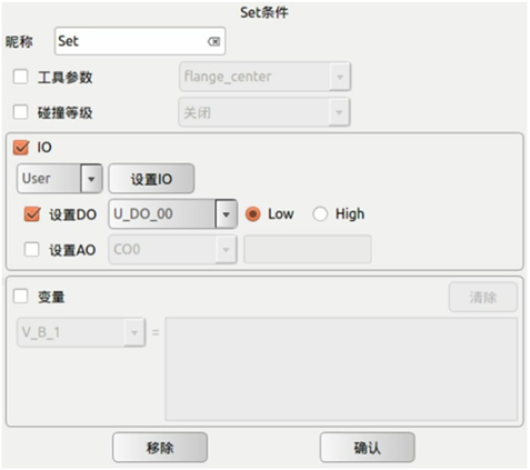• Click the input box to the right of the nickname to modify the command name. • Check Tool parameter: select a configured tool center. • Check Collision level to select a safety level. • The Set command is used to set the state of a DO/AO. • Check Variable: select a variable from the drop-down list below, and enter an expression on the right to assign a value to the selected variable; the expression follows C language operator rules. • Click Remove to remove the set command. • Click OK to confirm and save this command's state configuration. • When setting variables, a bool variable cannot be assigned 0 or 1; an int variable cannot be assigned true or false.	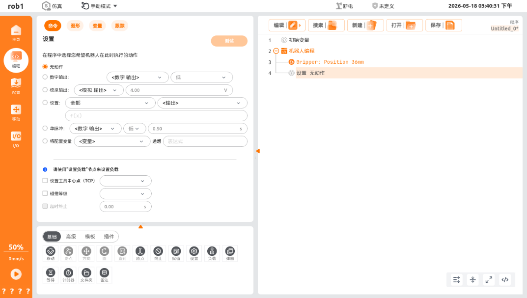• No action: no operation. • Digital output: set a digital output signal. • Analog output: set an analog output signal. • Set: set the expression for a digital output port or analog output port. Digital output ports support only true/false or 1/0, where Modbus ports support only 1/0. • Single pulse: set the duration for which the digital output port continuously outputs high/low level. • Increment configuration variable: configure the increment value of the selected variable. • Set Tool Center Point (TCP): select a TCP. For TCP creation and settings, see Tool Center Point. • Collision level: set the collision level. • Test: execute this node's settings once. When 【Set】 or 【Increment configuration variable by 1】 is selected, this node cannot be tested. • Timeout termination: when enabled (checked) with a non-zero time set, if the bus write operation is not completed within the set time, the program terminates immediately and pops up a runtime error. When unchecked or the time is set to 0.00s, it returns directly without checking whether the write succeeded.
Wait command	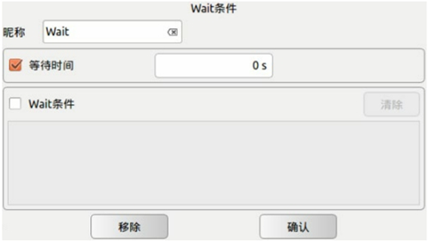The Wait command is used to wait for a time or a digital input signal. • Click the input box to the right of the nickname to modify the command name. • Check Wait time to set the waiting time; the time value is set by the user. • Check Wait condition to set the waiting mode by entering an expression. • Click Clear to clear the condition content. • Click OK to confirm and save the wait condition. • Click Remove to remove the wait command.	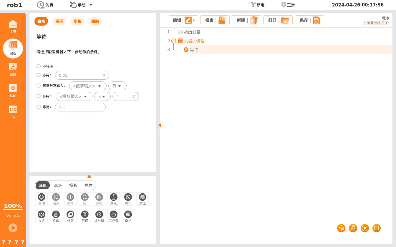The 【Wait】 command sets the wait time or digital input signal. • Do not wait: the robot does not wait. • Wait … seconds: the robot waits for the set time and then continues running. • Wait for digital signal input: waits to receive the set digital signal and then continues running. • Wait for analog signal input: waits to receive the set analog signal and then continues running. • Wait for expression: waits until the expression is true and then continues running.
Line comment command Block comment command	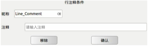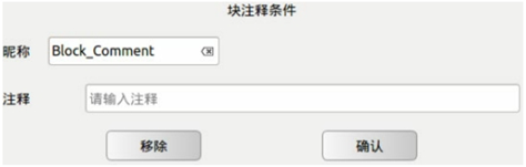Line Comment is a line-comment command that explains the program line below it. Block Comment is a block-comment command that explains the program block below it.	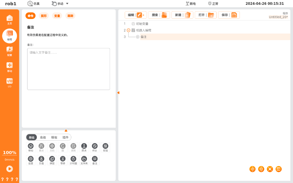The 【Remark】 command helps users record comment information; the remark text is not displayed while the program is running.
Popup command	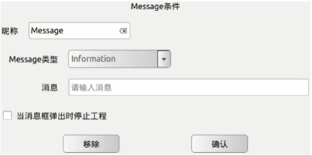Message is an information popup command that conveys status information to the user through a popup window. The popup command (Message) specifies a message that is displayed on the screen when the program reaches this command. • Click the input box to the right of the nickname to modify the command name. • You can select the message type. Click the Message type drop-down menu, which corresponds to Information, Warning, and Critical — three message types with different icon styles. • Click the blank input box to the right of the message to enter text conveying status information. • After the popup window is displayed, the robot waits for the user/operator to press the OK button in the window before continuing to run the program. • Check Stop project when the message box pops up; when an information window pops up, the project automatically stops. • Click Remove to delete the selected Message. • Click OK to confirm the state configuration and save it.	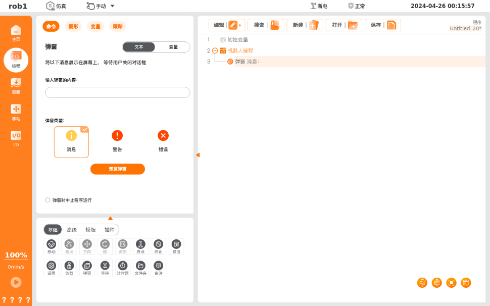The 【Popup】 command lets the user specify a message; when the program reaches this node, the message is displayed on the screen. • Text: enter the message text; click 【Preview Popup】 to view the popup effect. Text popups are of three types: Message, Warning, and Error. • Variable: select a variable; when the program reaches this node, a popup displays the variable's value and waits for the user to close the dialog. Variable popups are of three types: Message, Warning, and Error. • Pause the program when popping up: when checked, when the program reaches the 【Popup】 node, the popup message is displayed on the screen and the program's execution is paused.

1.5 Advanced Condition Feature Comparison

Feature	PE	ARCS
Thread control command	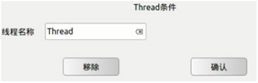Thread is a multi-thread control command. In a Thread program block, there must be a Loop command; within that Loop, parallel control with the main program can be implemented. Note: it is recommended to avoid using multiple threads as much as possible. If you must use multiple threads, pay attention to the parallel logic and timing matching between the main thread and auxiliary threads. • Click the input box to the right of the nickname to modify the command name. • Click Remove to delete the selected Thread. • Click OK to confirm the state configuration and save it.	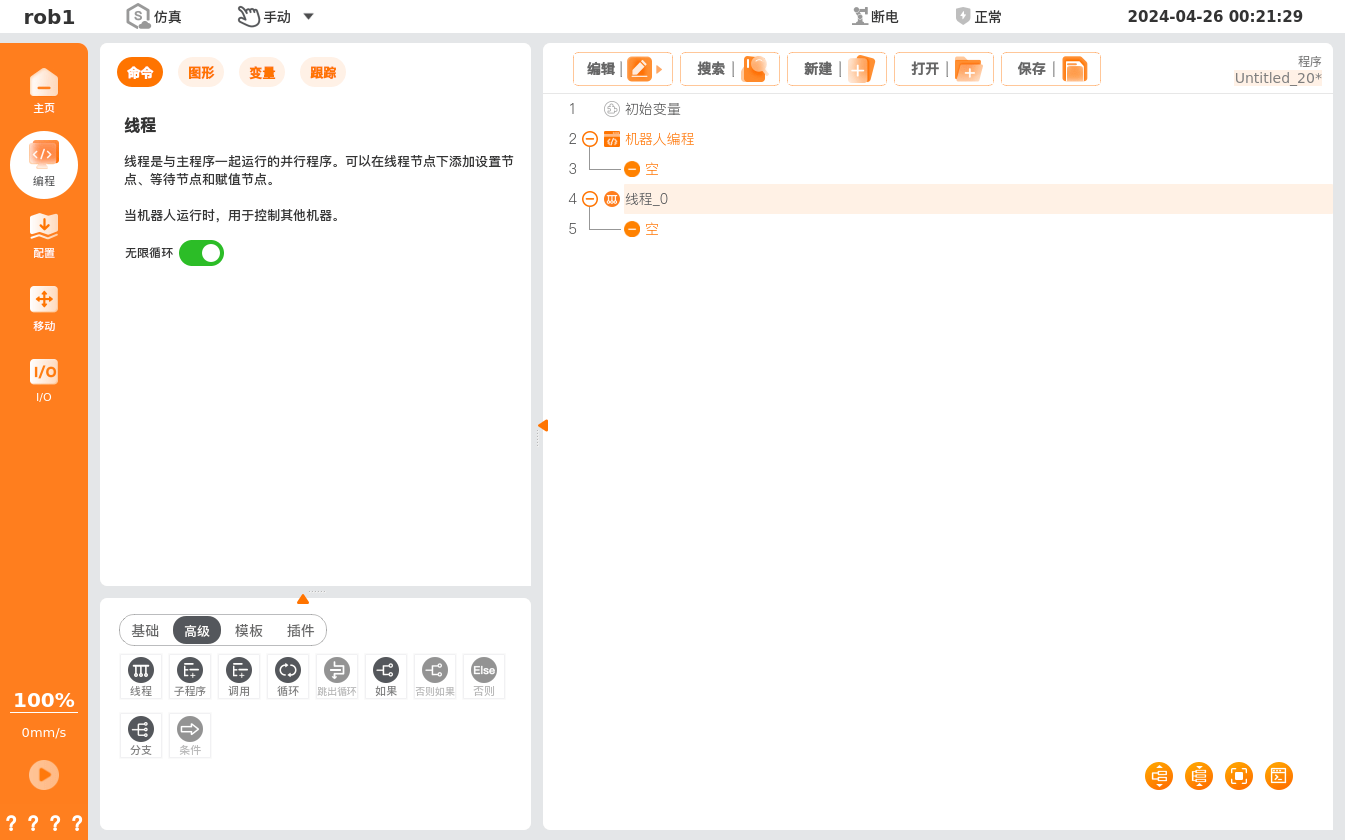The 【Thread】 command creates multiple threads, i.e., programs that can run in parallel with the main program. Threads can be used to control other external devices unrelated to the robot arm. Note: • Nodes unrelated to motion, such as Set, Wait, and Assignment, can be added under the thread node. • If motion-related nodes such as Move and Waypoint are added under the thread node, it may cause robot operation conflicts and other safety risks. • It is recommended to avoid using multiple threads as much as possible. If you must use multiple threads, pay attention to the parallel logic and timing matching between the main thread and auxiliary threads. • Infinite loop: when checked, the program in the thread can run in an infinite loop until the program is stopped.
Script command	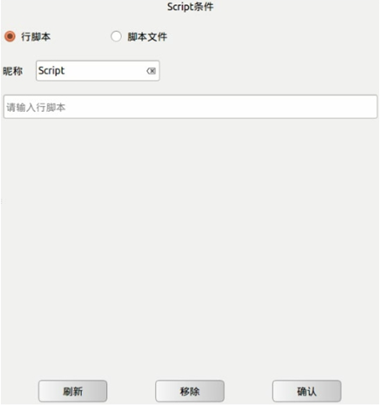Script is a script-editing command. In a Script, you can choose to add line scripts and script files. Click the input box to the right of the nickname to modify the command name. Click Line Script to add a line script; in the input box below, you can enter a single line of script control instruction. Click Script File to add a script file; you can select the script file to load from the file list. • Click Refresh as file update button to scan the current file save directory and update the display of file changes. • Click Remove to delete the selected Script command. • Click OK to confirm the state configuration and save it.	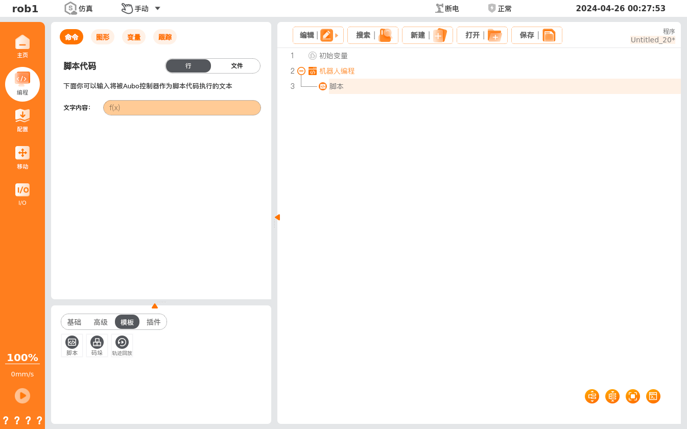The 【Script】 command adds a script line or a script file. • Line: enter text to be executed as script code via the editor. • File: open or save-as a script file, and perform operations such as edit, clear, and save-as on the opened script file.

1.6 Track Recording Feature Comparison

Feature	PE	ARCS
Record track	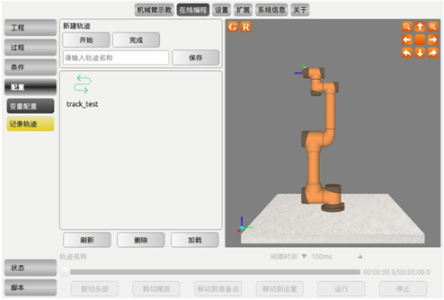New track: click the Start button to begin recording the robot arm's motion trajectory, click the Finish button to end recording, enter the track name in the input box, and click Save to complete the track recording. Track playback: select the track icon, click Load in the interface, long-press the Move to Ready Point button to move the robot arm to the initial position of the recorded track, then click Run to play back the track. Track pause: click Stop to pause the robot arm during playback. Resume after track pause: long-press Move to Ready Point to synchronize the robot arm to the current-progress pose, then click Run to resume track playback. Interval time: the track recording time unit is 100ms per waypoint; the interval time means how much time is used to play back these 100ms. For example, setting the interval time to 50ms plays the track at 2× speed, while setting it to 200ms plays it at 0.5× speed.	The 【Record】 interface can store the trajectory of the robot's motion over a period of time, and the stored trajectory can be added to a program.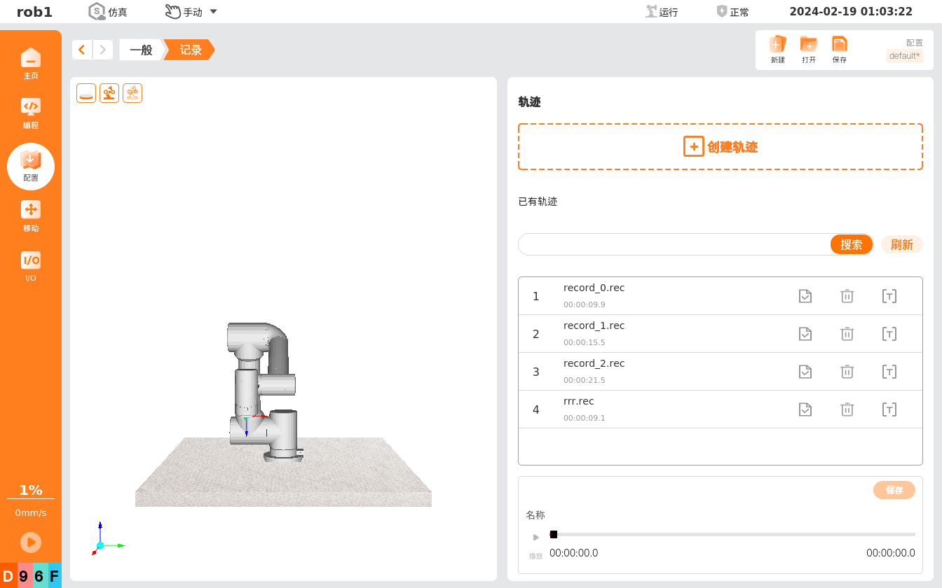 • Create track: click the 【Create Track】 button to enter the 【Move】 interface, operate the robot with the position/orientation control buttons, and the system begins recording the robot's running trajectory. After the run ends, click 【OK】, edit the track name, and save the track. • Search: search tracks by track name. • Refresh: refresh the track list. • Load: load a track. • Rename: rename the track file. • Delete: delete the track. • Play: play the currently loaded track. After clicking 【Play】, enter the 【Move】 interface, move the robot to the initial position, click 【OK】 to start playing the track, and 【Play】 changes to 【Pause】.
Call track recording command	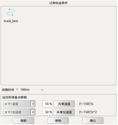The Record Track command is a track playback command. • Create or open a project file, and select Advanced Conditions in the toolbar. • Click Record Track in the properties window, and click Record Track in the project logic area. • Select the track icon in the properties window on its right and click OK to load the track recording into the project logic. • Interval time: the track recording time unit is 100ms per waypoint; the interval time means how much time is used to play back these 100ms. For example, setting the interval time to 50ms plays the track at 2× speed, while setting it to 200ms plays it at 0.5× speed. • The run-to-ready-point parameter input boxes at the bottom of the interface set the speed and acceleration of each joint when the robot arm moves to the ready point. After modifying, click the OK button. • Click Refresh as file update button to scan the current file save directory and update the display of file changes. • Click Remove to delete the Track_Record command in the project logic area.	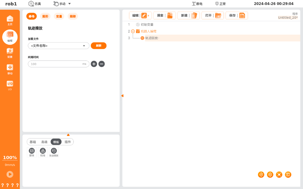The 【Track Playback】 command inserts a track file into the program. When the program reaches the track playback node, it plays the track file and the robot moves along the trajectory recorded in the file. A track file records the robot's motion trajectory and is generally stored in the installation configuration file. • Load file: click "Load File" or the icon and select a track file; track playback occurs when the program reaches this node. • Refresh: click to refresh the "Load File" drop-down menu. • Interval time: adjust the speed of track playback.

1.7 Variable Configuration Feature Comparison

Feature	PE	ARCS
Variable configuration	Variable settings currently support only bool, int, double, and pose variable types. The table shows all currently configured variables, including variable name, variable type, global hold, and variable value. When a variable is selected in the table, its information is displayed in the variable type drop-down list, the variable name input box, and the variable value selection/input options below. • bool: defines a bool variable whose value is true/false; click the variable value option to assign a value. • int: defines an integer variable whose value is an integer; enter the value in the cell after the variable value. • double: defines a double-precision variable whose value is a double-precision floating-point number; enter the value in the cell after the variable value. • pose: defines a position-type variable whose value is the robot waypoint information; click the 【Set Waypoint】 button behind the variable value cell to jump to the robot teaching interface; after completing the waypoint setting, click 【OK】 to complete the variable assignment. The variable pose is represented by 3 groups (13 values total): the first 3 values are position parameters in meters; the middle 4 values are orientation parameters displayed as a quaternion in radians; the last 6 values are the 6 joint parameters in radians. You can provide only the position and orientation parameters, or only the joint parameters; when both are provided, the joint parameters take priority, and any parameters not provided must be replaced with the value 0. Global hold: checking Global hold means the variable value is persisted to the database; if Global hold is not checked, the variable value remains the initial value set when the variable was added each time the program restarts. 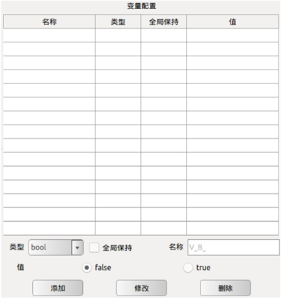• Add variable: select a variable type, enter the variable name and value, and click Add. Note: variable names must be unique and can contain only digits, letters, and underscores. • Modify variable: select a variable in the table and click Modify to change the variable name and value. Note: the variable type cannot be modified. • Delete variable: select a variable in the table and click Delete.	The 【Variables】 interface lets you create configuration variables and set their initial values; click 【Save】 in the configuration management toolbar to save to the configuration file. While the program is running, this interface updates the configuration variables' state in real time. Variables in the ARCS system are divided into the following three types: • Configuration variable: this variable can be used across multiple programs. As long as the currently loaded configuration file is not switched, the variable name and value are continuously saved; it is a retentive variable. • Program variable: this variable applies only to the running program, and its value is lost after the program stops; it is a conventional program variable. For details, see "Programming Tab - Basic Program Nodes - Assignment". • Script variable: this variable comes from a script file and can be assigned different variable types. Script variables do not appear in the 【Programming】 or 【Configuration】 interfaces. Robot programs use script variables to store information about waypoints. 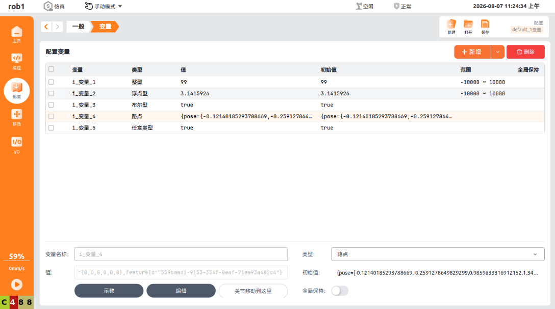Click 【Add】 in the Variables interface to start adding a variable. • Variable name: the name of the new variable; it can be modified as needed. • Type: supports 【Integer】, 【Floating-point】, 【Boolean】, 【Waypoint】, and 【Any type】. • Value: the value of the variable type; it can be changed in the program through assignment and other operations.  - Integer: integer-type number, supports custom value lower/upper limits; the configured limits must not exceed the range: -10000 ≤ value range ≤ 10000.  - Floating-point: decimal-type number, using 64-bit double-precision floating point with up to 16 significant digits; supports custom value lower/upper limits.  - Boolean: logical-state type, supporting only two values: true and false.  - Waypoint: a composite robot point data type containing Cartesian pose, joint angles, TCP offset, and orientation feature information. You can modify it by clicking 【Teach】 or 【Edit】 at the bottom of the page, and click 【Joint Move Here】 to move the robot to the waypoint variable's position.  - Any type: can store data of multiple types, including integer, floating-point, boolean, and waypoint. • Initial value: after creating or modifying a variable in the Variables interface, the variable's corresponding value is synchronized as the initial value. • Global hold: controls whether the 【initial value】 or the 【value】 changed in the program is used when the variable is loaded in the program.  - Enable 【Global hold】: the 【Initial value】 input box is hidden; when 【value】 is modified during program execution, the modified value is persisted. After restarting the teach pendant, the variable loads the last-saved 【value】.  - Disable 【Global hold】: the 【value】 entered when creating the variable is synchronously saved as the 【initial value】; during program execution the 【value】 can be modified, but the 【initial value】 remains fixed. After the teach pendant restarts, the variable loads the 【initial value】 as the current 【value】. • Delete variable: select the target variable on the left side of the Variables interface, then click 【Delete】 in the upper-right corner to delete it. • Modify variable: select the target variable in the Variables interface, then modify the parameters in the area below; the parameter-setting rules are the same as when creating the parameter.

1.8 Timer Feature Comparison

Feature	PE	ARCS
Insert timer	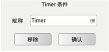The Timer command is a timing command that measures the running time of nodes in the project file. • Click the blank input box to the right of the nickname to modify the command name. • Click Remove to delete the selected line comment command. • Click OK to confirm the state configuration and save it.	The 【Timer】 command records the program's running time.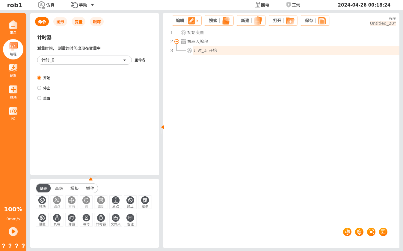 In the 【Timer】 interface drop-down box, you can select a timer, or select 【New】 in the drop-down box to create a new timer. The default timer name is "timer_0"; each new timer increments the default value by 1. Rename: click to customize the timer name. 【Timer】 status: • Start: the timer starts counting. • Stop: the timer stops counting. • Reset: the timer resets.
Timer status display	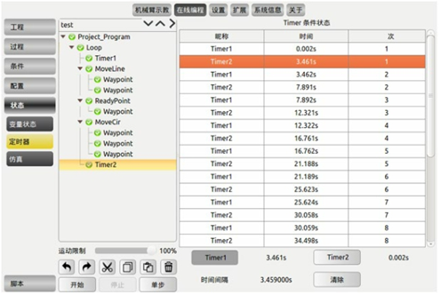Select Online Programming in the menu bar and Status-Timer in the toolbar to view the timer status display. • The nickname corresponds to the command name in the project file. • Time is the time taken from the program start point to this Timer command. • Times indicates the number of times this Timer command has been executed in the program file. • Timer1 and Timer2 are the corresponding times displayed when a certain Timer command is selected. • Time interval is the interval between the selected Timer and the previously selected Timer. • Note: the display of timer1 and timer2 is related to the order in which condition names in the list are clicked, based on the gray state of the buttons, and is unrelated to the display order of the time names.	The value of the program's running time is displayed in the 【Variables】 interface.

1.9 Project Log Feature Comparison

Feature	PE	ARCS
Project log	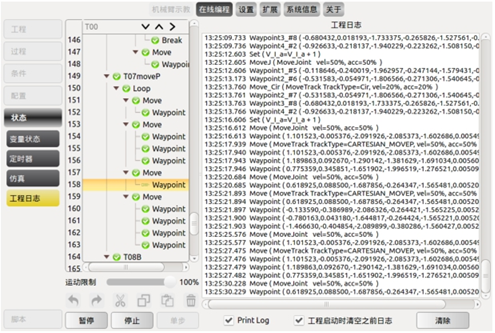The project log can display the project's real-time running status. When you click Start to run a program, the interface automatically switches to the project log.	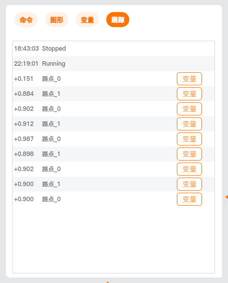The 【Trace】 tab displays in real time the start of the current project and the running time of program nodes; click the 【Variables】 button in the record list to view detailed information, which facilitates program debugging.

1.10 Script File Feature Comparison

Feature	PE	ARCS
Script file	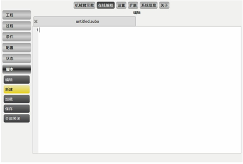Select Online Programming in the menu bar and Script in the toolbar to edit, create, load, and save script files. Note: when editing script files, the code must conform to LUA syntax; otherwise the script file cannot be saved.	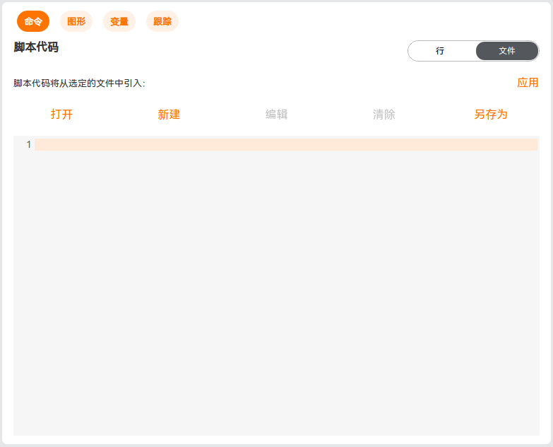Before editing a script, first open a saved script or 【Save As】 the script, then click 【Edit】 to edit the script; otherwise the script cannot be edited. The script editor has a built-in syntax checker: when correct script code is entered, the editor background is white; otherwise it is yellow. Only correct script code can be saved to the script file.

---

2 Script Interfaces

2.1 Math Module

Feature	PE	ARCS
Convert Euler angles to quaternion	Function prototype: {oriW,oriX,oriY,oriZ} rpy2quaternion({oriRX,oriRY,oriRZ}) Parameters: Euler angles (radians) Returns: The quaternion converted from the Euler angle parameters Example: quaternion = rpy2quaternion({0.611, 0.785, 0.960})	Function prototype: rpyToQuaternion(rpy: table) -> table Parameters: rpy Euler angles Returns: Quaternion Example: rpyToQuaternion({0.611, 0.785, 0.960})
Convert quaternion to Euler angles	Function prototype: {oriRX,oriRY,oriRZ} quaternion2rpy({oriW,oriX,oriY,oriZ}) Parameters: Quaternion Returns: The Euler angles (radians) converted from the quaternion parameter Example: rpy = quaternion2rpy({0.834722, 0.0780426, 0.451893, 0.304864})	Function prototype: quaternionToRpy(quat: table) -> table Parameters: quat quaternion Returns: Euler angles Example: rpy = quaternionToRpy({0.834722, 0.0780426, 0.451893, 0.304864})

2.2 Motion Module

Feature	PE	ARCS
Joint motion	Function prototype: void move_joint({double joint1Angle, double joint2Angle, double joint3Angle, double joint4Angle, double joint5Angle, double joint6Angle}, bool isBlock) Parameters: • {joint1Angle ~ joint6Angle} the six joint angle values in radians of the target waypoint • isBlock whether to block Returns: None Example: move_joint({-2.05177, -0.400292, 1.19625, 0.0285152, 1.57033, -2.28774}, true)	Function prototype: moveJoint(q: table, a: number, v: number, blend_radius: number, duration: number) -> nil Parameters: • Non-blocking motion • q joint angles, unit rad • a acceleration, unit rad/s²; the maximum value can be obtained through the getJointMaxAccelerations() interface in the RobotConfig class • v speed, unit rad/s; the maximum value can be obtained through the getJointMaxSpeeds() interface in the RobotConfig class • blend_radius blend radius, unit m • duration running time, unit s. Normally, when speed and acceleration are given, the trajectory's running time can be determined. To extend the trajectory's running time, set the duration parameter. duration can extend the trajectory motion time but cannot shorten it. When duration = 0, it means no running time is specified, and the running time is calculated from speed and acceleration. If duration is not 0, the values of a and v are ignored Returns: • 0 success • AUBO_BAD_STATE(1) the current safety mode is not in Normal, ReducedMode, or Recovery state • AUBO_QUEUE_FULL(2) the planning queue is full • AUBO_BUSY(3) the previous instruction is still executing • -AUBO_BAD_STATE(-1) the thread is detached or terminated, task_id not found, or the current robot mode is not Running • -AUBO_TIMEOUT(-4) interface call timed out • -AUBO_INVL_ARGUMENT(-5) the length of the parameter array q is less than the current robot arm's degrees of freedom • AUBO_REQUEST_IGNORE(13) the length of the parameter array q is too short and no stop is needed at that point Example: moveJoint({-2.05177, -0.400292, 1.19625, 0.0285152, 1.57033, -2.28774}, 0.3, 0.3, 0, 0)
Linear motion	Function prototype: void move_line({double joint1Angle, double joint2Angle, double joint3Angle, double joint4Angle, double joint5Angle, double joint6Angle}, bool isBlock) Parameters: Exactly the same as the move_joint function parameters Returns: None Example: move_line({-0.000003, -0.127267, -1.321122, 0.376934, -1.570796, -0.000008}, true)	Function prototype: moveLine(pose: table, a: number, v: number, blend_radius: number, duration: number) -> nil Parameters: • Non-blocking motion • pose target pose • a acceleration (if the position change is less than 1mm and the orientation change is greater than 1e-4 rad, this acceleration is treated as angular acceleration in rad/s²; otherwise it is linear acceleration in m/s²); the maximum value can be obtained through the getTcpMaxAccelerations() interface in the RobotConfig class • v speed (if the position change is less than 1mm and the orientation change is greater than 1e-4 rad, this speed is treated as angular velocity in rad/s; otherwise it is linear velocity in m/s); the maximum value can be obtained through the getTcpMaxSpeeds() interface in the RobotConfig class • blend_radius blend radius, unit m, with a value between 0.001 and 1 • duration running time, unit s. Normally, when speed and acceleration are given, the trajectory's running time can be determined. To extend the trajectory's running time, set the duration parameter. duration can extend the trajectory motion time but cannot shorten it. When duration = 0, it means no running time is specified, and the running time is calculated from speed and acceleration. If duration is not 0, the values of a and v are ignored Returns: • 0 success • AUBO_BAD_STATE(1) the current safety mode is not in Normal, ReducedMode, or Recovery state • AUBO_QUEUE_FULL(2) the trajectory queue is full • AUBO_BUSY(3) the previous instruction is still executing • -AUBO_BAD_STATE(-1) the thread is detached or terminated, task_id not found, or the current robot mode is not Running • -AUBO_TIMEOUT(-4) interface call timed out • -AUBO_INVL_ARGUMENT(-5) the length of the parameter array pose is less than the current robot arm's degrees of freedom • AUBO_REQUEST_IGNORE(13) the path length of the parameter array pose is too short and no stop is needed at that point Example: moveLine({0.58815, 0.0532, 0.62391, 2.46, 0.479, 1.619}, 1.3, 1.0, 0, 0)
Get current waypoint	Function prototype: get_current_waypoint(void) Returns a nested structure of type table: • pos = {x, y, z} position • ori = {w, x, y, z} orientation (quaternion) • joint = {j1, j2, j3, j4, j5, j6} joint angles Parameters: None Returns: Real-time waypoint position, orientation, and joint angles as a table Example: realPoint = get_current_waypoint()	Function prototype: getJointPositions() -> table Gets the robot arm's joint angles Parameters: None Returns: Robot arm joint angles Example: JointPositions = getJointPositions() Function prototype: getToolPose() -> table Gets the tool-end pose (without TCP offset) Parameters: None Returns: The tool-end pose, in the form (x,y,z,rx,ry,rz) Example: ToolPose = getToolPose()
Inverse kinematics solution	Function prototype: {joint1Angle, joint2Angle, joint3Angle, joint4Angle, joint5Angle, joint6Angle} get_target_pose(bool isMulSol, ikRefPoint, toolEndPos, toolEndOri, enableEndRotate, endRotateAngle, toolPos, toolOri, coordCalibrateMethod, point1, point2, point3, toolEndPositionForCalibCoord) Parameters: • isMulSol whether to return multiple solutions (optional parameter, default false. When true, multiple solution sets are returned; when false or omitted, a single solution set is returned) • ikRefPoint the joint angles of the inverse-solution reference point • toolEndPos / toolEndOri tool end position and orientation • enableEndRotate whether to enable end rotation • endRotateAngle end rotation angle • toolPos / toolOri tool position and orientation • coordCalibrateMethod coordinate system calibration method • point1 / point2 / point3 calibration point joint angles • toolEndPositionForCalibCoord tool end position for the calibration coordinate system Returns: The joint angles {joint1Angle ~ joint6Angle} solved through inverse kinematics based on the specified position, orientation, tool, and user coordinate system parameters; returns false if the inverse solution fails Example: joint = get_target_pose({0, 0, -0.131415}, {0.707114, 0.000014, 0.7071, 0.000007}, true, d2r(20), {0.1, 0.2, 0.3}, {1.0, 0.0, 0.0, 0.0}, CoordCalibrateMethod.zOzy, {-0.000003, -0.127267, -1.321122, 0.376934, -1.570796, -0.000008}, {-0.186826, -0.164422, -1.351967, 0.383250, -1.570795, -0.186831}, {-0.157896, 0.011212, -1.191991, 0.367593, -1.570795, -0.157901}, {0.1, 0.2, 0.3})	Function prototype: inverseKinematics(qnear: table, pose: table) -> table, int Inverse kinematics solution: input the TCP pose and reference joint angles, output the joint angles Parameters: • qnear reference joint angles • pose TCP pose Returns: The joint angles and whether the inverse solution is valid. The first return value is the inverse solution result, and the second is the inverse solution error code: • 0 success • -1 the robot arm state is incorrect (not fully initialized; try calling again) • -5 the input reference joint angles or TCP pose are invalid (dimension error) • -23 the inverse solution calculation does not converge; calculation error • -24 the inverse solution calculation exceeds the robot's maximum limit • -25 there is an error in the inverse solution input configuration • -26 the inverse solution Jacobian matrix calculation failed • -27 the target point has analytical solutions, but none satisfy the solution-selection conditions • -28 the inverse solution returns an unknown error type If the error code is not 0, the first return value is the input reference joint angles qnear Example: joint, ik_result = inverseKinematics({0, 0, 0, 0, 0, 0}, {0.81665, -0.20419, 0.43873, -3.135, 0.004, 1.569})

Feature	PE	ARCS
Add waypoint	Function prototype: void add_waypoint({double joint1Angle, double joint2Angle, double joint3Angle, double joint4Angle, double joint5Angle, double joint6Angle}) Adds a waypoint to the global waypoint list, serving the move_track function Parameters: Type table, six joint angle values in radians Returns: None Example: add_waypoint({-0.000003, -0.127267, -1.321122, 0.376934, -1.570796, -0.000008})	Function prototype: pathBufferAppend(name: string, waypoints: table) -> nil Adds waypoints to the path buffer Parameters: • name the name of the path buffer • waypoints waypoints Returns: • Returns 0 on success • Returns error codes on failure: -AUBO_INVL_ARGUMENT, -AUBO_BAD_STATE Example: pathBufferAppend("traje_name", {{-0.000000, 0.000009, -0.000001, 0.000002, 0.000002, 0.000000}, {-0.000001, 0.000010, -0.000002, 0.000000, 0.000003, 0.000002}})
Clear waypoint list	Function prototype: void clear_global_waypoint_list(void) Clears the global waypoint list Parameters: None Returns: None Example: clear_global_waypoint_list()	Function prototype: pathBufferFree(name: string) -> nil Frees the path buffer Parameters: name the name of the buffered path Returns: • Returns 0 on success • Returns error codes on failure: -AUBO_INVL_ARGUMENT, -AUBO_BAD_STATE Example: pathBufferFree("traje_name")
Track motion	Function prototype: void move_track(MoveTrackType trackType, bool isBlock) Executes track motion based on the global waypoint list (added through the add_waypoint function) Parameters: • trackType track type (moveP, B-spline, etc.) • isBlock whether to block Returns: None Example: move_track(MoveTrackType.ARC_CIR, true)	Function prototype: movePathBuffer(name: string) -> nil Executes the buffered path Parameters: name the name of the buffered path Returns: • Returns 0 on success • Returns error codes on failure: -AUBO_INVL_ARGUMENT, -AUBO_BAD_STATE Example: movePathBuffer("traje_name") Function prototype: moveCircle(via_pose: table, end_pose: table, a: number, v: number, blend_radius: number, duration: number) -> nil Adds arc motion Parameters: • via_pose the pose of the intermediate point of the arc motion • end_pose the pose of the end point of the arc motion • acceleration (if the position change between via_pose and the previous waypoint is less than 1mm and the orientation change is greater than 1e-4 rad, this acceleration is treated as angular acceleration in rad/s^2; otherwise it is linear acceleration in m/s^2) • speed (if the position change between via_pose and the previous waypoint is less than 1mm and the orientation change is greater than 1e-4 rad, this speed is treated as angular velocity in rad/s; otherwise it is linear velocity in m/s) • blend_radius blend radius, unit m, with a value between 0.001 and 1 • duration running time, unit s. Normally, when speed and acceleration are given, the trajectory's running time can be determined. To extend the trajectory's running time, set the duration parameter. duration can extend the trajectory motion time but cannot shorten it. When duration = 0, it means no running time is specified, and the running time is calculated from speed and acceleration. If duration is not 0, the values of a and v are ignored Returns: • Returns 0 on success • Returns error codes on failure: -AUBO_INVL_ARGUMENT, -AUBO_BAD_STATE Example: moveCircle({0.440164,-0.00249391,0.398658,2.45651,0,1.5708},{0.440164,0.166256,0.297599,2.45651,0,1.5708},1.2,0.25,0,0)

Feature	PE	ARCS
Set blend radius	Function prototype: void set_blend_radius(double blendRadius) Sets the blend radius (i.e., the corner radius) Parameters: blendRadius is the blend radius, in meters Returns: None Example: set_blend_radius(0.01)	Function prototype: moveLine(pose: table, a: number, v: number, blend_radius: number, duration: number) -> nil Function prototype: moveJoint(q: table, a: number, v: number, blend_radius: number, duration: number) -> nil The blend radius is set directly in linear motion and joint motion
Set collision level	Function prototype: void set_robot_collision_class(int collisionClass) Sets the collision level Parameters: collisionClass 0~10 Returns: None Example: set_robot_collision_class(6)	Function prototype: setCollisionLevel(level: number) -> nil Sets the collision sensitivity level; the larger the value, the more sensitive Parameters: • level collision sensitivity level • 0: turns off collision detection • 1~9: collision sensitivity level Returns: • Returns 0 on success • Returns error codes on failure: AUBO_BUSY, AUBO_BAD_STATE, -AUBO_INVL_ARGUMENT, -AUBO_BAD_STATE Example: setCollisionLevel(6)
Set tool kinematics parameters	Function prototype: void set_tool_kinematics_param({double posX, double posY, double posZ}, {double oriW = 1, double oriX = 0, double oriY = 0, double oriZ = 0}) Sets the tool kinematics parameters; the orientation can be omitted Parameters: Two tables: • The first table is position (required) • The second table is orientation (optional) Returns: None Example: set_tool_kinematics_param({0.1, 0.2, 0.3})	Function prototype: setTcpOffset(offset: table) -> nil Sets the current TCP offset. The TCP offset is represented as (x, y, z, rx, ry, rz). x, y, z are the position offsets of the tool center point (TCP) relative to the flange center in the base coordinate system, in m. rx, ry, rz are the orientation offsets of the tool center point (TCP) relative to the flange center in the base coordinate system, expressed as ZYX Euler angles in rad Parameters: offset the current TCP offset, in the form (x, y, z, rx, ry, rz) Returns: • Returns 0 on success • Returns error codes on failure: AUBO_BUSY, AUBO_BAD_STATE, -AUBO_INVL_ARGUMENT, -AUBO_BAD_STATE Example: setTcpOffset({0.1, 0.2, 0.3, 0.0, 0.0, 0.0})
Get tool kinematics parameters	Function prototype: {double toolEndPosX, toolEndPosY, toolEndPosZ}, {double toolEndOriW, toolEndOriX, toolEndOriY, toolEndOriZ} get_tool_kinematics_param(string toolName) Gets the tool kinematics parameters Parameters: toolName tool name, which must match the tool name in the teach pendant tool calibration interface Returns: The tool end position parameters and tool end orientation parameters Example: get_tool_kinematics_param("toolName")	Function prototype: getTcpOffset() -> table Parameters: Gets the current TCP offset. The TCP offset is represented as (x, y, z, rx, ry, rz). x, y, z are the position offsets of the tool center point (TCP) relative to the flange center in the base coordinate system, in m. rx, ry, rz are the orientation offsets of the tool center point (TCP) relative to the flange center in the base coordinate system, expressed as ZYX Euler angles in rad Returns: The current TCP offset, in the form (x, y, z, rx, ry, rz) Example: TcpOffset = getTcpOffset()
Set tool dynamics parameters	Function prototype: void set_tool_dynamics_param(double payload, {double gravityCenterX, double gravityCenterY, double gravityCenterZ}, {double inertiaXX = 0, double inertiaXY = 0, double inertiaXZ = 0, double inertiaYY = 0, double inertiaYZ = 0, double inertiaZZ = 0}) Sets the tool dynamics parameters; payload and center-of-gravity xyz are required, and inertia can be omitted Parameters: • payload payload, unit kg • center-of-gravity table • inertia table Returns: None Example: set_tool_dynamics_param(3, {0.1, 0.2, 0.3})	Function prototype: setPayload(m: number, cog: table, aom: table, inertia: table) -> nil Sets the payload Parameters: • m mass, unit: kg • cog center of gravity, unit: m, in the form (CoGx, CoGy, CoGz) • aom direction of the moment axis, unit: rad, in the form (rx, ry, rz) • inertia inertia, unit: kg*m^2, in the form (Ixx, Iyy, Izz, Ixy, Ixz, Iyz) or (Ixx, Ixy, Ixz, Iyx, Iyy, Iyz, Izx, Izy, Izz) Returns: • Returns 0 on success • Returns error codes on failure: AUBO_BUSY, AUBO_BAD_STATE, -AUBO_INVL_ARGUMENT, -AUBO_BAD_STATE Example: setPayload(3, {0.1, 0.2, 0.3}, {0,0,0}, {0,0,0,0,0,0,0,0,0})

Feature	PE	ARCS
Pause motion	Function prototype: void robot_pause(void) Pauses the robot arm's motion. It can be called only when the robot arm is in motion Parameters: None Returns: None Example: robot_pause()	Function prototype: pause() -> number Pauses the interpreter Parameters: None Returns: None Example: pause()
Resume motion	Function prototype: void robot_continue(void) Resumes the robot arm's motion. It can be called only when the robot arm is paused Parameters: None Returns: None Example: robot_continue()	Function prototype: resume() -> number Resumes the interpreter Parameters: None Returns: None Example: resume()
Emergency stop	Function prototype: void robot_fast_stop(void) Emergency-stops the robot arm. It can be called only when the robot arm is in motion Parameters: None Returns: None Example: robot_fast_stop()	Function prototype: abort() -> number Terminates the robot's run. If you only want to stop the run, you can call the RuntimeMachine::stop interface. If the runtime is in the Running state when the script runs, it terminates the runtime; if the runtime is in the Stopped state and the robot is moving, it stops the robot's movement; if force control is enabled at this time, the robot stops force control Parameters: None Returns: None Example: abort()

Feature	PE	ARCS
Pose transformation	Function prototype: {Fca_PosX, Fca_PosY, Fca_PosZ}, {Fca_OriW, Fca_OriX, Fca_OriY, Fca_OriZ} pose_trans({Fba_PosX, Fba_PosY, Fba_PosZ}, {Fba_OriW, Fba_OriX, Fba_OriY, Fba_OriZ}, {Fcb_PosX, Fcb_PosY, Fcb_PosZ}, {Fcb_OriW, Fcb_OriX, Fcb_OriY, Fcb_OriZ}) Parameters: • {Fba_PosX, Fba_PosY, Fba_PosZ} the position of coordinate system a in coordinate system b • {Fba_OriW, Fba_OriX, Fba_OriY, Fba_OriZ} the orientation of coordinate system a in coordinate system b • {Fcb_PosX, Fcb_PosY, Fcb_PosZ} the position of coordinate system b in coordinate system c • {Fcb_OriW, Fcb_OriX, Fcb_OriY, Fcb_OriZ} the orientation of coordinate system b in coordinate system c Returns: The position and orientation of coordinate system a in coordinate system c Example: target_pos, target_ori = pose_trans({0.2, 0.5, 0.1}, {1.0, 0, 0, 0}, {0.2, 0.5, 0.6}, {1.0, 0, 0, 0})	Function prototype: poseTrans(pose_from: table, pose_from_to: table) -> table The first parameter p_from is used to transform the second parameter p_from_to, and the result is returned. This means the result is the pose obtained by starting from the p_from coordinate system and then moving p_from_to within that coordinate system. If the pose is treated as a transformation matrix: • T_world->to = T_world->from * T_from->to • Given the pose of B relative to A and the pose of C relative to B, find the pose of C relative to A Parameters: • pose_from the starting pose (space vector) • pose_from_to the pose change relative to the starting pose (space vector) Returns: The result pose (space vector) Example: pose_trans = poseTrans({0.2, 0.5, 0.1, 1.57, 0, 0}, {0.2, 0.5, 0.6, 1.57, 0, 0})
Pose inversion	Function prototype: {Fab_PosX, Fab_PosY, Fab_PosZ}, {Fab_OriW, Fab_OriX, Fab_OriY, Fab_OriZ} pose_inv({Fba_PosX, Fba_PosY, Fba_PosZ}, {Fba_OriW, Fba_OriX, Fba_OriY, Fba_OriZ}) Parameters: • {Fba_PosX, Fba_PosY, Fba_PosZ} the position of coordinate system a in coordinate system b • {Fba_OriW, Fba_OriX, Fba_OriY, Fba_OriZ} the orientation of coordinate system a in coordinate system b Returns: The position and orientation of coordinate system b in coordinate system a Example: pose_inverse_pos, pose_inverse_ori = pose_inv({0.2, 0.5, 0.1}, {1.0, 0, 0, 0})	Function prototype: poseInverse(pose: table) -> table Parameters: pose tool pose (space vector) Returns: The inverse transform of the tool pose (space vector) Example: pose_inverse = poseInverse({0.2, 0.5, 0.1, 1.57, 0, 3.14})

Code example 1: pose_trans — move the robot arm 100mm along the Z-axis of the flange coordinate system while rotating 90° around the Z-axis of the flange coordinate system

-- Move to the ready point
moveJoint({-3e-06, -0.176728, -1.93304, -0.807424, -1.5708, -8e-06}, 0.3, 0.3, 0, 0)
sleep(2)

-- Pose of the target point in the flange coordinate system [x,y,z,rx,ry,rz]
pose_wrt_tool = {0, 0, 0.1, 0, 0, 1.5708}

-- Pose of the flange coordinate system in the base coordinate system
current_joint = getJointPositions()

pose, fk_result = forwardToolKinematics(current_joint)

-- Calculate the pose of the target point in the base coordinate system via poseTrans
pose_trans = poseTrans(pose, pose_wrt_tool)
-- Calculate the inverse kinematics solution
joint, ik_result = inverseKinematics(current_joint, pose_trans)

-- Move there in a straight line
moveLine(pose_trans, 1.3, 1.0, 0)

Code example 2: pose_inv — given the pose of the target point in the base coordinate system and the pose of the user coordinate system in the base coordinate system, obtain the pose of the target point in the user coordinate system

-- The known pose of the target point in the base coordinate system
pose_wrt_base = {-0.3, -0.3, 0.4, 3.14159, 2.05266e-06, -1.57079}

-- The known pose of the feature coordinate system in the base coordinate system
feature_wrt_base = {-0.3, -0.3, 0.3, 0, 0, 0}

-- Calculate the pose of the base coordinate system in the feature coordinate system via poseInverse
base_wrt_feature = poseInverse(feature_wrt_base)

-- Calculate the pose of the target point in the feature coordinate system via poseTrans
pose_trans = poseTrans(base_wrt_feature, pose_wrt_base)

-- Print
textmsg("---------- pose wrt feature--------------- ")
textmsg("pos [" .. tostring(pose_trans[1]) .. ", " .. tostring(pose_trans[2]) .. ", " .. tostring(pose_trans[3]) .. "]")
textmsg("rpy [" .. tostring(pose_trans[4]) .. ", " .. tostring(pose_trans[5]) .. ", " .. tostring(pose_trans[6]) .. "]")

2.3 Internal Module

Feature	PE	ARCS
Set robot arm body IO	Function prototype: void set_robot_io_status(RobotIOType ioType, string name, double value) Sets the robot arm body IO state Parameters: • ioType indicates the IO type, an enumeration type • name IO name • value IO state value Returns: None Example: set_robot_io_status(RobotIOType.RobotBoardUserDI, "U_DO_00", 1)	Function prototype: setStandardAnalogOutput(index: number, value: number) -> nil Sets the standard analog output value Parameters: • index indicates the pin of the IO port; pin numbering starts from 0, e.g., 0 is the first pin • value analog output value Returns: • Returns 0 on success • Returns error codes on failure: AUBO_REQUEST_IGNORE, AUBO_BUSY, AUBO_BAD_STATE, -AUBO_INVL_ARGUMENT, -AUBO_BAD_STATE Example: setStandardAnalogOutput(0, 5.4) Function prototype: setStandardDigitalOutput(index: number, value: boolean) -> nil Sets the standard digital output value Parameters: • index indicates the pin of the IO port; pin numbering starts from 0, e.g., 0 is the first pin • value output value Returns: • Returns 0 on success • Returns error codes on failure: AUBO_REQUEST_IGNORE, AUBO_BUSY, AUBO_BAD_STATE, -AUBO_INVL_ARGUMENT, -AUBO_BAD_STATE Example: setStandardDigitalOutput(0, true)
Get robot arm body IO	Function prototype: double get_robot_io_status(RobotIOType ioType, string name) Gets the robot arm body IO state Parameters: • ioType indicates the IO type, an enumeration type • name IO name Returns: The state value of the corresponding IO, of type double Example: a = get_robot_io_status(RobotIOType.RobotBoardUserDI, "U_DI_00") print(a)	Function prototype: getStandardAnalogInput(index: number) -> number Gets the standard analog input value Parameters: index indicates the pin of the IO port; pin numbering starts from 0, e.g., 0 is the first pin Returns: The standard analog input value Example: getStandardAnalogInput(0) Function prototype: getStandardDigitalInput(index: number) -> boolean Gets the standard digital input value Parameters: index indicates the pin of the IO port; pin numbering starts from 0, e.g., 0 is the first pin Returns: Returns true for high level; returns false for low level Example: getStandardDigitalInput(0)
Set tool power voltage	Function prototype: void set_tool_power_voltage(ToolPowerType toolPowerType) Sets the tool power voltage Parameters: toolPowerType tool power voltage enumeration value; see the enumeration types section Returns: The state value of the corresponding IO, of type double Example: set_tool_power_voltage(ToolPowerType.OUT_12V)	Function prototype: setToolVoltageOutputDomain(domain: number) -> nil Parameters: domain the tool-end power voltage value, with three selectable levels: • 0 means 0V • 12 means 12V • 24 means 24V Returns: • Returns 0 on success • Returns error codes on failure: AUBO_REQUEST_IGNORE, AUBO_BUSY, AUBO_BAD_STATE, -AUBO_INVL_ARGUMENT, -AUBO_BAD_STATE Example: setToolVoltageOutputDomain(24)

2.4 Modbus

Feature	PE	ARCS
Get Modbus IO state	Function prototype: double get_modbus_io_status(string ioName) Gets the Modbus IO state Parameters: ioName Modbus IO name (defined by Teach Pendant Extension → Peripherals → Modbus → IO Config) Returns: Modbus IO state Example: get_modbus_io_status("M_DO_0")	Function prototype: modbusGetSignalStatus(signal_name: string) -> number Parameters: signal_name the name of the signal whose value is to be obtained Returns: • For digital signals: 1 or 0 • For register signals: the register value represented as an integer. If the value is -1, the signal does not exist Example: var0 = modbusGetSignalStatus("Modbus_0")
Set Modbus IO state	Function prototype: void set_modbus_io_status(string ioName, double ioValue) Sets the Modbus IO state Parameters: • ioName Modbus IO name (defined by Teach Pendant Extension → Peripherals → Modbus → IO Config) • ioValue IO value Returns: None Example: set_modbus_io_status("M_DO_0", 1)	Function prototype: modbusSetOutputSignal(signal_name: string, value: number) -> nil Parameters: • signal_name an output register signal added in advance • value must be a valid integer in the range 0-65535 Returns: Modbus IO state Example: modbusSetOutputSignal("Modbus_0", 0)

2.5 TCP Server

Feature	PE	ARCS
Listen on port	Function prototype: void listen(int port) TCP server listens on the port Parameters: port port number Returns: None Example: tcp.server.listen(8888)	Function prototype: socket.bind(address, port [, backlog]) Parameters: • address local address • port local port • backlog (optional) the maximum length of the pending connection queue passed to the listen method, defaulting to 32 Returns: A TCP server object bound to the specified local address and port and ready to accept client connections Example: local server = assert(socket.bind(ip, port))
Check client connection	Function prototype: bool is_connected(string IP) Checks whether the client with the given IP has established a connection with the local server Parameters: IP IP address Returns: Returns true if the IP in the parameter is already connected to the TCP server; otherwise returns false Example: while (tcp.server.is_connected(ip) ~= true) do sleep(1) end print("connection succeeded")	Function prototype: server:accept() Parameters: None (this method is called on the server object and takes no additional parameters) Returns: • On successful connection: returns a client object representing the connection • On timeout: returns nil, followed by the error string 'timeout' • On other errors: returns nil, followed by a message describing the error Example: local client = server:accept()
Receive data	Function prototype: string recv_str_data(string IP) The local server receives data from the client with the given IP as a string Parameters: IP IP address Returns: The received data Example: recv = tcp.server.recv_str_data("127.0.0.1")	Function prototype: client:receive([pattern [, prefix]]) Parameters: pattern (optional) read mode, following the Lua file I/O format: • '*a': reads data from the socket until the connection closes, without line-ending conversion • '*l': reads a line of text from the socket, ending with an LF character (default mode) • number: reads the specified number of bytes • prefix (optional) is concatenated in front of the received data before returning Returns: • On success: returns the received content • On error: returns nil followed by an error message ('closed' or 'timeout'), plus the partial result transferred Example: local recv = client:receive(3)
Send data	Function prototype: void send_str_data(string IP, string msg) The local server sends a message to the client with the given IP as a string Parameters: • IP IP address • msg the message to send Returns: None Example: tcp.server.send_str_data("127.0.0.1", "Hello world")	Function prototype: client:send(data [, i [, j]]) Parameters: • data the string to send • i (optional) the starting position of the substring, consistent with string.sub • j (optional) the ending position of the substring, consistent with string.sub Using i and j, a substring of data can be selected for sending Returns: • On success: returns the index of the last byte sent (when i is 1 or omitted, this is the total number of bytes sent) • On error: returns nil followed by an error message ('closed' or 'timeout'), plus the index of the last byte sent Example: client:send("Hello ")
Close server	Function prototype: void close(void) The local server stops listening and disconnects all established connections Parameters: None Returns: None Example: tcp.server.close()	Function prototype: close() Parameters: None Returns: None Example: server:close()

Code example 3: TCP server — receive data from the client in ASCII form; if the received data is "end", exit the program

local socket = require("socket")

-- Define the printTable function (must be placed before it is called)
function printTable(tbl, level, keyName)
    if type(tbl) ~= "table" then
        return
    end
    if next(tbl) == nil then
        return
    end
    level = level or 1
    keyName = keyName or ""

    local indent = string.rep("   ", level)

    if keyName ~= "" then
        textmsg(indent .. keyName .. " = {")
    else
        textmsg(indent .. "{")
    end

    for k, v in pairs(tbl) do
        if type(v) == "table" then
            printTable(v, level + 1, tostring(k))
        else
            textmsg(string.format("%s   %s = %s", indent, tostring(k), tostring(v)))
        end
    end

    textmsg(indent .. "}")
end

-- Server configuration
local ip = "0.0.0.0"   -- Listen on all NICs
local port = 8866

local server = assert(socket.bind(ip, port))
textmsg("Listening on " .. ip .. ":" .. port)

local client = server:accept()
textmsg("Client connected")

client:send("Hello ")
client:send("world")

-- Receive loop
while true do
    client:settimeout(1)          -- 1 second timeout
    local recv = client:receive(3)

    if recv then
        textmsg("recv from port " .. port .. " :")
        -- Convert the string to a byte table and pass it to printTable
        local byteTable = { string.byte(recv, 1, #recv) }
        printTable(byteTable)

        if recv == "end" then
            textmsg("break")
            break
        end
    end
end

client:close()
server:close()
textmsg("tcp server end")

2.6 TCP Client

Feature	PE	ARCS
Connect to server	Function prototype: void connect(string IP, int port) Connects to the TCP server with the specified IP and port Parameters: • IP IP address • port port number Returns: None Example: tcp.client.connect("127.0.0.1", 7777)	Function prototype: connect(address, port) Parameters: • address IP address or hostname • port port number, which must be an integer in the range [1..64K) Returns: • On error: returns nil followed by a string describing the error • On success: returns 1 Example: local client1 = assert(socket.connect(ip, port1))
Receive data	Function prototype: string recv_str_data(string IP, int port) Receives data sent from the TCP server with the specified IP and port as a string Parameters: IP IP address Returns: The data sent from the server Example: recv = tcp.client.recv_str_data("127.0.0.1", "7777") print(recv)	Function prototype: client:receive([pattern [, prefix]]) Parameters: pattern (optional) read mode, following the Lua file I/O format: • '*a': reads data from the socket until the connection closes, without line-ending conversion • '*l': reads a line of text from the socket, ending with an LF character (default mode) • number: reads the specified number of bytes • prefix (optional) is concatenated in front of the received data before returning Returns: • On success: returns the received content • On error: returns nil followed by an error message ('closed' or 'timeout'), plus the partial result transferred Example: local recv = client:receive(3)
Send data	Function prototype: void send_str_data(string IP, int port, string msg) Sends data to the TCP server with the specified IP and port as a string Parameters: • IP IP address • port port number • msg the message to send Returns: None Example: tcp.client.send_str_data("127.0.0.1", 7777, "Hello world")	Function prototype: client:send(data [, i [, j]]) Parameters: • data the string to send • i (optional) the starting position of the substring, consistent with string.sub • j (optional) the ending position of the substring, consistent with string.sub Using i and j, a substring of data can be selected for sending Returns: • On success: returns the index of the last byte sent (when i is 1 or omitted, this is the total number of bytes sent) • On error: returns nil followed by an error message ('closed' or 'timeout'), plus the index of the last byte sent Example: client:send("Hello ")
Disconnect	Function prototype: void disconnect(string IP, int port) Disconnects from the TCP server with the specified IP and port Parameters: • IP IP address • port port number Returns: None Example: tcp.client.disconnect("127.0.0.1", 7777)	Function prototype: close() Parameters: None Returns: None Example: server:close()

Code example 4: TCP client — connect to two TCP servers with the same IP address but different port numbers, receive data in ASCII form, and exit upon receiving "end"

local socket = require("socket")

key = ""
function printTable(table, level)
    if (#table == 0) then
        return
    end
    level = level or 1
    local indent = ""
    for i = 1, level do
        indent = indent .. " "
    end

    if key ~= "" then
        textmsg(indent .. key .. " " .. "=" .. " " .. "{")
    else
        textmsg(indent .. "{")
    end

    key = ""
    for k, v in pairs(table) do
        if (type(v) == "table") then
            key = k
            printTable(v, level + 1)
        else
            local content = string.format("%s%s = %s", indent .. "", tostring(k), tostring(v))
            textmsg(content)
        end
    end
    textmsg(indent .. "}")
end


-- =========================================================
-- tcp client
-- =========================================================

local ip    = "192.168.18.1"
local port1 = 9601
local port2 = 9602

-- Establish two TCP connections
local client1 = assert(socket.connect(ip, port1))
local client2 = assert(socket.connect(ip, port2))

-- Port 1: first send the string "Hello", then send the byte sequence of "world"
client1:send("Hello")

local world = {
    string.byte("world", 1), string.byte("world", 2), string.byte("world", 3),
    string.byte("world", 4), string.byte("world", 5)
}
-- Concatenate the byte table into a string and send it (LuaSocket can only send strings)
local worldStr = string.char(table.unpack(world))
client1:send(worldStr)

-- Port 2: first send the byte sequence of "Hello", then send the string " world"
local hello = {
    string.byte("Hello", 1), string.byte("Hello", 2), string.byte("Hello", 3),
    string.byte("Hello", 4), string.byte("Hello", 5)
}
local helloStr = string.char(table.unpack(hello))
client2:send(helloStr)
client2:send(" world")

textmsg("string.byte : " .. string.byte("end"))

recv = {}

-- Non-blocking polling: set a very short timeout; returns nil if nothing is received
client1:settimeout(0)
client2:settimeout(0)

while (true) do
    -- Port 1: byte data
    local recv1 = client1:receive(3)
    -- Port 2: string data
    local recv2 = client2:receive(3)

    -- Check whether port 1 received "end"
    if (recv1 ~= nil) and (#recv1 == 3) then
        local byteTable = { string.byte(recv1, 1, #recv1) }
        if (string.format("%c%c%c", byteTable[1], byteTable[2], byteTable[3]) == "end") then
            textmsg("from port1 break")
            break
        end
        textmsg(string.format("recv data from port %d,data length %d", port1, #byteTable))
        printTable(byteTable)
    end

    -- Check whether port 2 received "end"
    if (recv2 ~= nil) and (#recv2 == 3) then
        if (recv2 == "end") then
            textmsg("from port2 break")
            break
        end
        textmsg(string.format("recv data from port %d,data length %d", port2, #recv2))
        textmsg(recv2)
    end
end

client1:close()
client2:close()
socket.sleep(1)

textmsg("tcp client end")

---

3 System Configuration

3.1 Robot Arm Settings

3.1.1 Fixed Pose Feature Comparison

Feature	PE	ARCS
Select initial pose	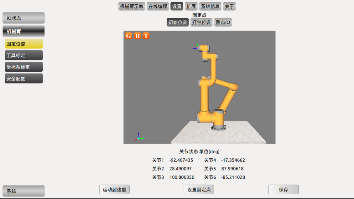Operation: Click 【Set Fixed Point】 → move the robot arm by operating the robot teaching interface or using drag teaching → set the robot's initial position → sync it to 【Initial Pose】 at the bottom of the teaching interface.	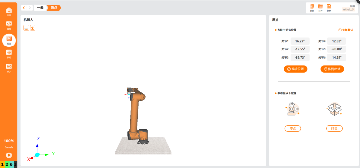Operation: Set the robot's initial position through 【Edit Position】; you can move the robot arm by operating the teaching interface or using drag teaching, and after setting, it is synced to 【Origin】 in the Move interface.
Select packing pose	Operation: Click 【Move Here】 → move the robot arm to the packing pose; Click 【Set Fixed Point】 → modify the packing pose.	Operation: The packing pose does not support modification by default; Long-press the 【Auto】 button in the Move interface to move to the packing pose.
Initial position IO settings	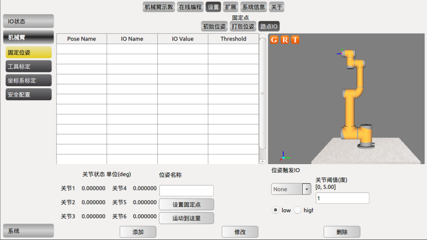Configuration steps: Select a DO from the drop-down menu → check 【high】 → click Save IO; After the robot arm moves to the initial position, the selected DO outputs a signal; Enter the joint threshold → click Save IO.	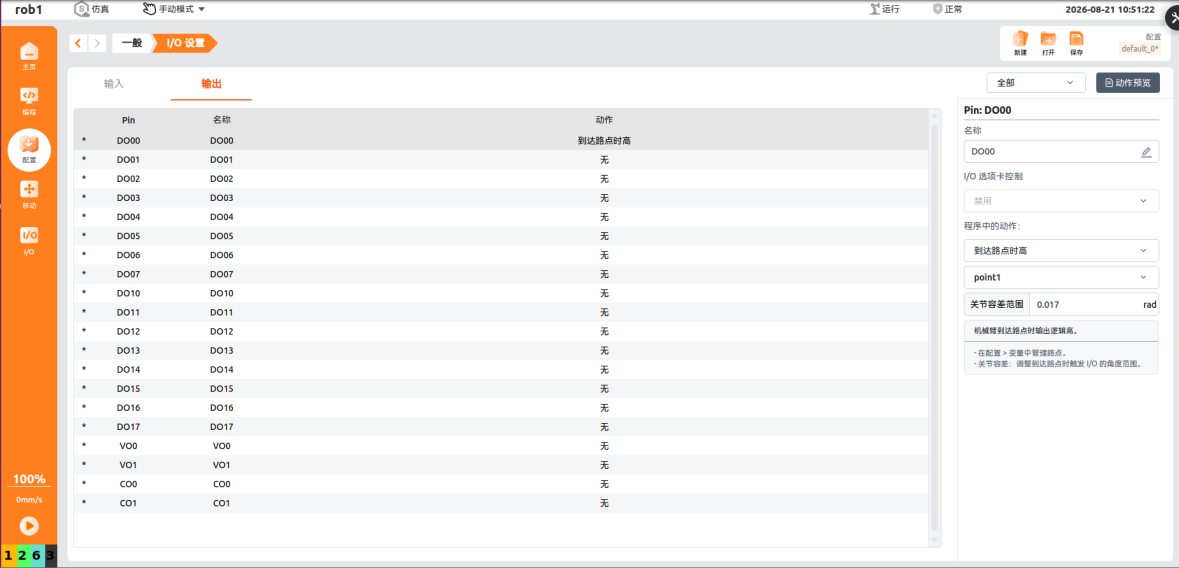Configuration steps: Select a DO in the I/O interface and configure 【High when reaching waypoint】 and the corresponding waypoint variable; after the robot arm reaches the waypoint variable, the DO outputs a signal; setting a joint tolerance range is supported.

3.1.2 Tool Calibration Feature Comparison

Feature	PE	ARCS
Kinematics calibration	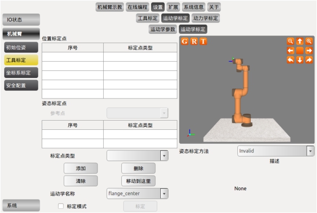Tool kinematics calibration includes position calibration and orientation calibration; it is recommended to determine the position calibration points first, then the orientation calibration points. Position calibration: • Requires ≥4 waypoints (mandatory) • All position calibration points must satisfy that the tool end position remains unchanged relative to the robot arm base coordinate system • Operation: Settings → Tool Calibration → Kinematics Calibration → select 【Position Calibration Point】 as the calibration point type → Add → determine the position point in the teaching interface Orientation calibration: • Requires exactly 2 waypoints (not counting reference points) • Optional; if not calibrated, the tool orientation is the same as the flange orientation • Type 1 (with reference point): xOxy, yOyz, zOzx • Type 2 (without reference point): TxRBz_TxyPBzAndTyABnz, TyRBz_TyzPBzAndTzABnz, TzRBz_TzxPBzAndTxABnz Kinematics parameter settings: 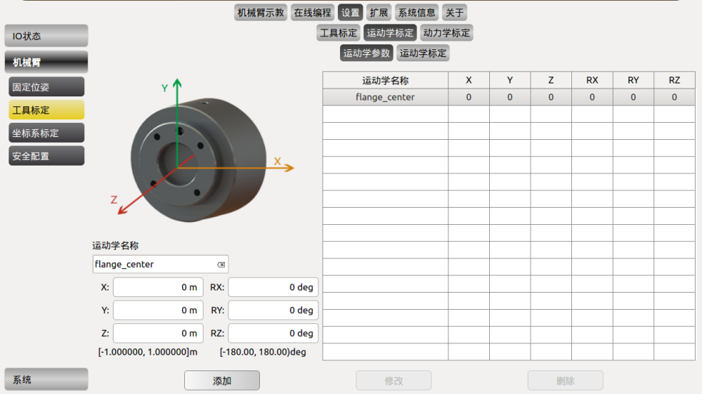• Kinematics parameters are the distance and orientation parameters of the tool relative to the wrist 3 tool end • After calibration, the parameters are automatically added to the data display area • Enter the kinematics name → click 【Add】 • Manual parameter entry is supported • Select a parameter in the list → 【Modify】 or 【Delete】 • Note: flange_center is a system default parameter and cannot be modified or deleted	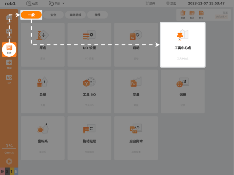Position calibration: Enter via 【Configuration → General → Tool Center Point → Add → Position → Measure】; after teaching 4 waypoints, the system automatically calculates the deviation between the TCP and the flange center. Orientation calibration: Enter via 【Direction → Measure】; select the coordinate system and teach the tool orientation, and the system automatically calculates and fills in the direction parameters. 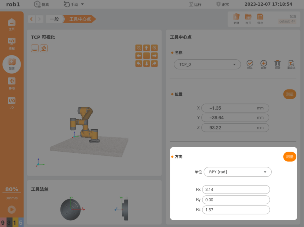Parameter management: The calculated result is automatically filled into the 【Direction】 parameter; no manual entry is required.
Dynamics calibration	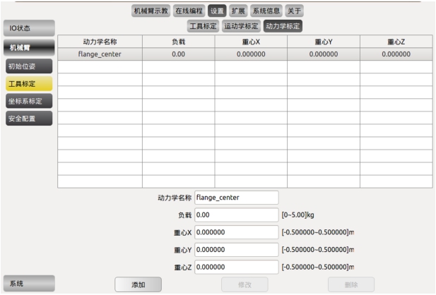Operation: • Enter the tool dynamics name, tool payload, and tool center-of-gravity parameters → click 【Add】 to complete calibration • Modify: select the item to modify → enter the value → click 【Modify】 • Delete: select the item to delete → click 【Delete】 • Note: flange_center is a system default parameter and cannot be modified or deleted	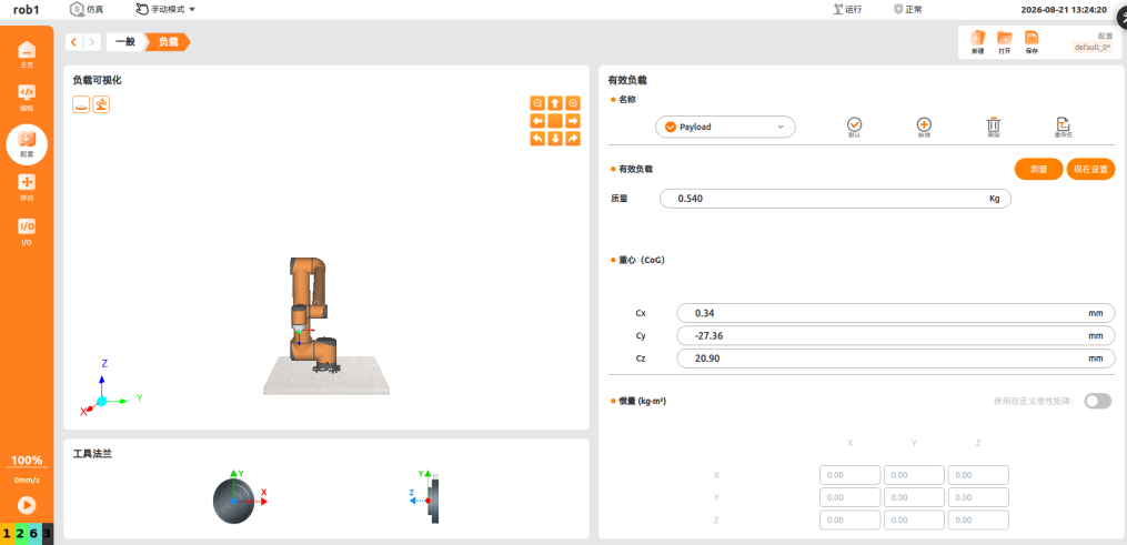Function button descriptions: • Current default: the current default payload • Default: set as the default payload • Add: add a payload • Rename: rename the currently selected payload • Delete: delete the selected payload • Set now: immediately apply the currently set payload • Measure: payload identification wizard  - Method 1: manually enter the payload and center-of-gravity values  - Method 2: use the payload identification wizard to automatically calculate the payload and center of gravity (CoG)

3.1.3 Coordinate System Calibration Feature Comparison

Feature	PE	ARCS
Coordinate system calibration	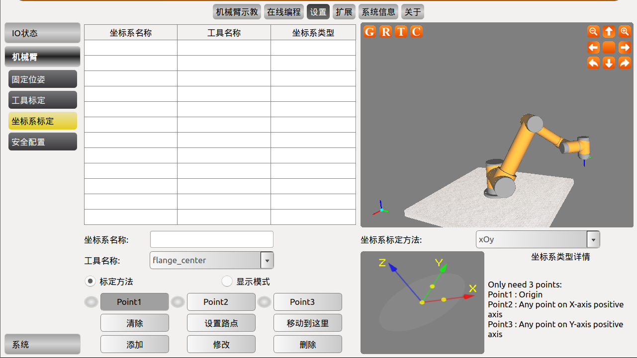Operation flow: Select the coordinate system type from the 【Coordinate System Calibration Method】 drop-down menu → select 【Calibration Method】 → set Point1/Point2/Point3 in order (click 【Set Waypoint】 to enter the teaching interface for calibration) → enter 【Coordinate System Name】 → click 【Add】 to save. Function description: • Modify: select the coordinate system → click 【Modify】 → you can modify Point1-3 and the name • Delete: select the coordinate system → click 【Delete】 • Clear: clear the calibration results of Point1-3 • Display mode: displays the values of the three waypoints of the calibrated coordinate system; after selecting the coordinate system, it enters automatically, and clicking Point1-3 displays the corresponding waypoints in the simulation interface • Move here: in calibration mode or display mode, select any one of Point1-3 and click 【Move Here】 to move to the corresponding waypoint	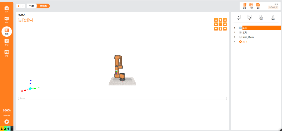A new coordinate system is built in three ways — point, line, and plane — and the coordinate system is located by the TCP position. Build via point: 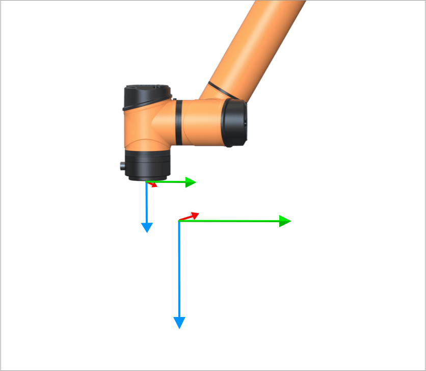• Teach the origin position of the new coordinate system via the TCP; the coordinate system axis directions are the same as the TCP directions • Usually used to define the robot's safety boundary or global main configuration • Supports 【Joint Move Here】 or 【Linear Move Here】 to return to the constructed pose Build via line: 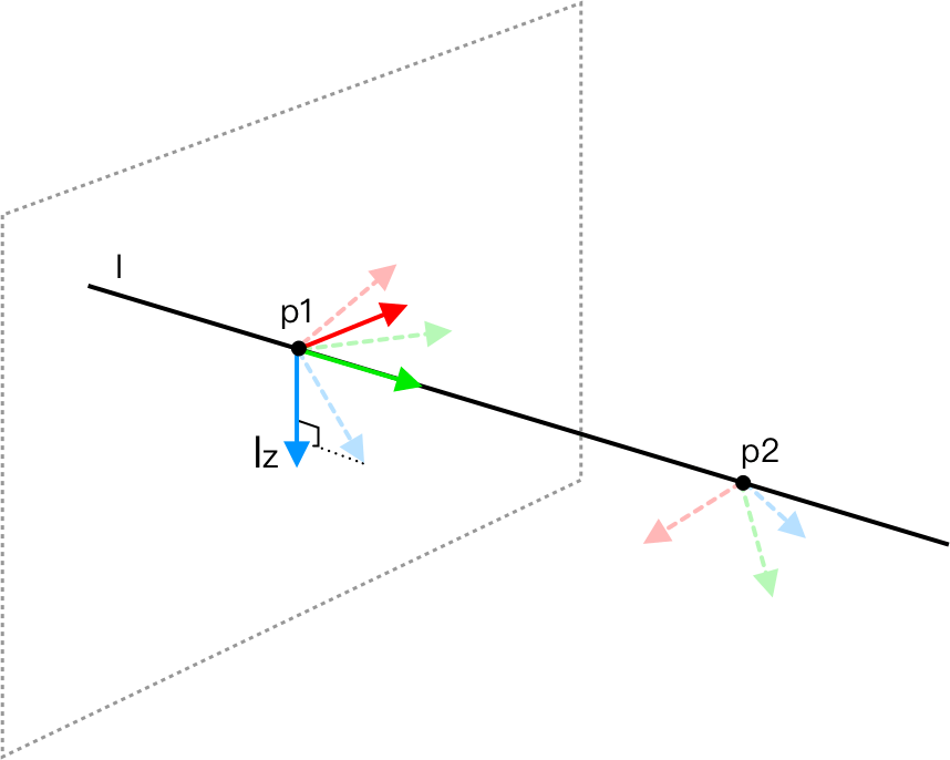• The origin is defined by the first point; the Y-axis is the axis from the first point to the second point; the Z-axis is the projection of the first point's Z-axis onto the plane perpendicular to the line Build via plane (three-point calibration method): 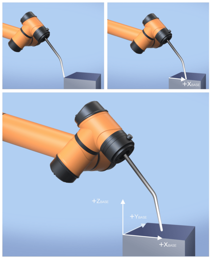• The origin is defined by the first point; the X-axis is the axis from the first point to the second point; the third point lies on the XY plane, and the Z-axis is perpendicular to the XY plane, satisfying the right-hand rule • Generally used when a high-precision frame is required

3.1.4 Robot Arm Safety Configuration Feature Comparison

Feature	PE	ARCS
Basic conditions	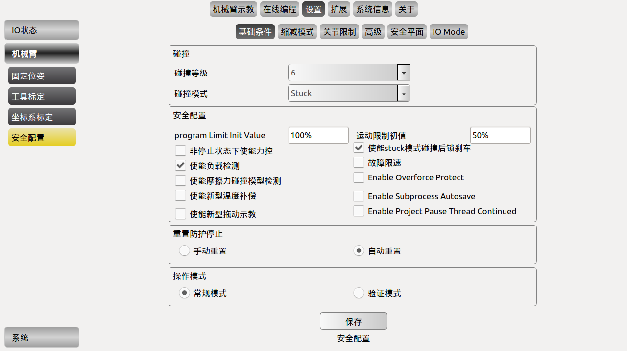Collision level: • There are 1-10 safety levels • The higher the level, the smaller the force required to stop after collision detection • Level 6 is the default level Collision mode: • Free: after a collision, enters drag-teaching mode • Stuck: after a collision, holds the current position and cannot be dragged Motion limit initial value: • The limit value for the project's running speed • Takes effect after restarting the software once configuration is complete • It is initialized only once after the software starts; afterwards, the changed value prevails Reset protective stop: • Manual reset: the protection can be released only when the protective-reset external input signal is active • Automatic reset: ignores external input signals; the protection is automatically released when the protective-stop signal is inactive	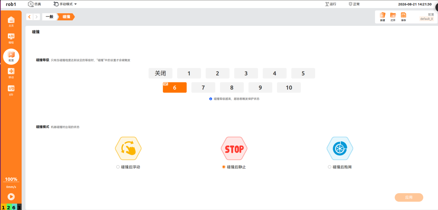Collision level: • There are 10 safety levels • The smaller the value, the higher the level, and the greater the force required to trigger a collision event • The system default collision level is 6 Collision mode: • Float after collision: stops and enters drag-teaching mode; the robot can be manually dragged to a safe position • Stand still after collision: stops and remains still • Brake after collision: stops and engages the brake to remain still (only for robots with firmware version 1.*.*) Navigation bar: Can set the default running speed Safety input signal configuration: 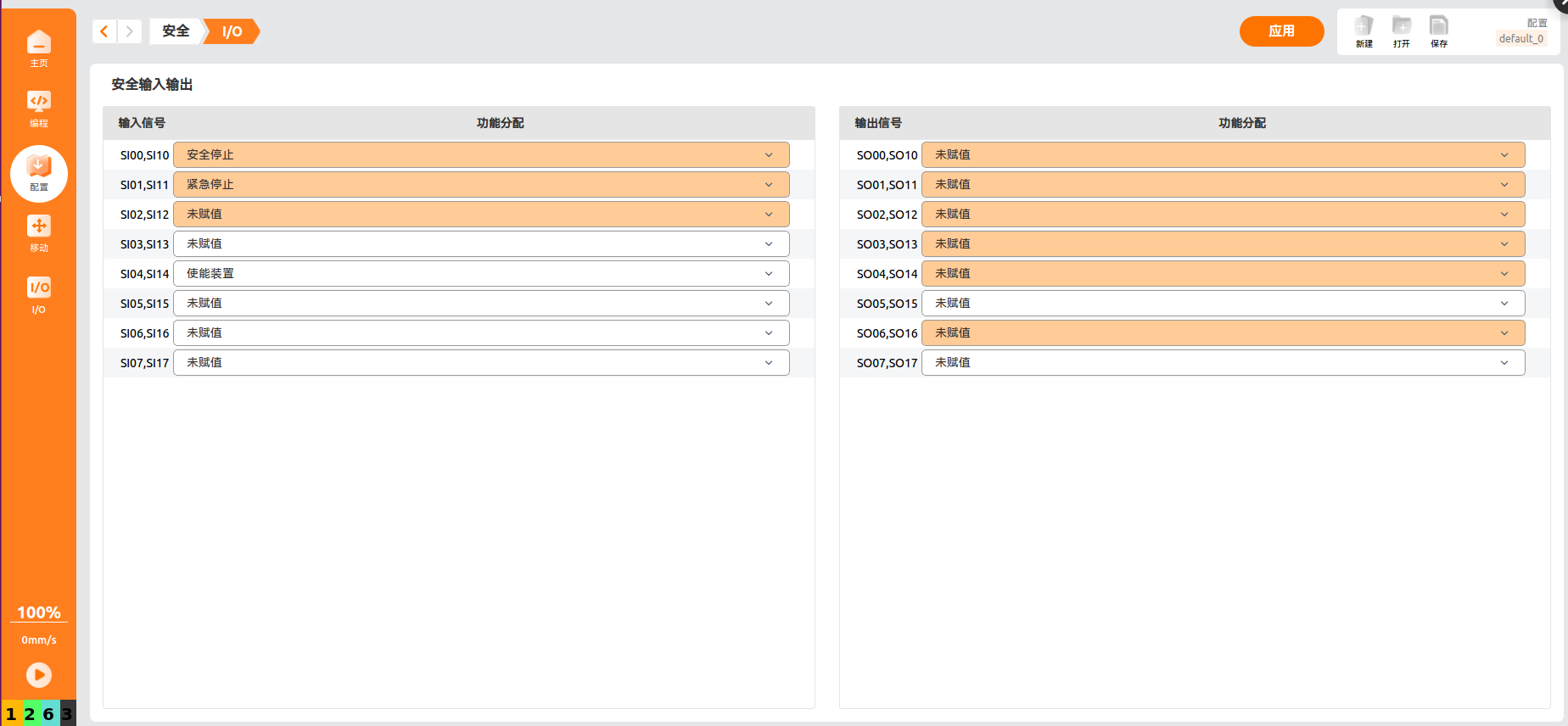Manual reset → set safety stop and safety reset separately: • Safety stop (trigger mode: logic low): level-triggered; safety stop is triggered when the signal is set to logic low. Can be used together with safety reset • Safety reset (trigger mode: rising edge): edge-triggered; after the safety stop recovers, the safety stop is released on the rising edge. Must be configured together with safety stop Automatic reset → set the enabling device: • Enabling device (trigger mode: logic low): a logic-high signal keeps normal operation, and logic low triggers a safety stop. Dual-channel I/O must receive valid signals simultaneously; effective in manual mode
Reduced mode	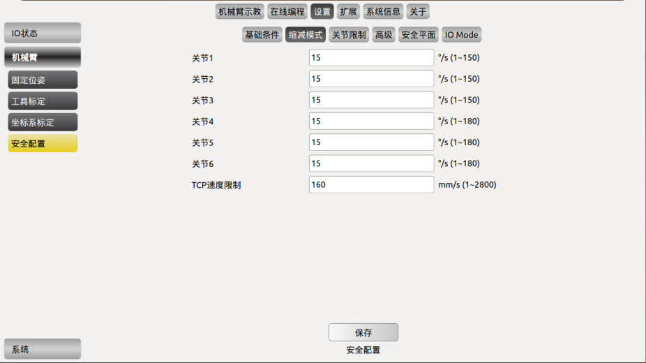After this mode is activated, the robot arm's motion speed is limited: • Joint space: joints 1/2/3 1~150°/s, joints 4/5/6 1~180°/s • Cartesian space: TCP speed limit 1~2800mm/s 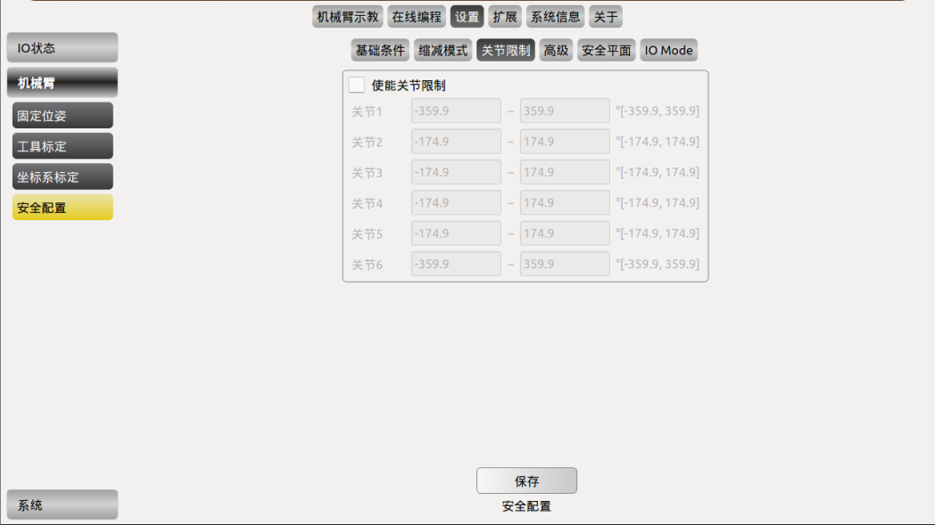Joint limit description: Joint limits default to the maximum limits the joints can reach; the user can limit the angle of each joint during operation. If a set angle exceeds the actual range, the value automatically reverts to the default. If the robot arm runs beyond the set angle, it stops and displays a warning, and the joint limits must be re-adjusted. Excessive angle overshoot can cause a power-off; after recovery, the joint limits revert to the default, and the robot arm must be moved to a suitable position before re-setting them.	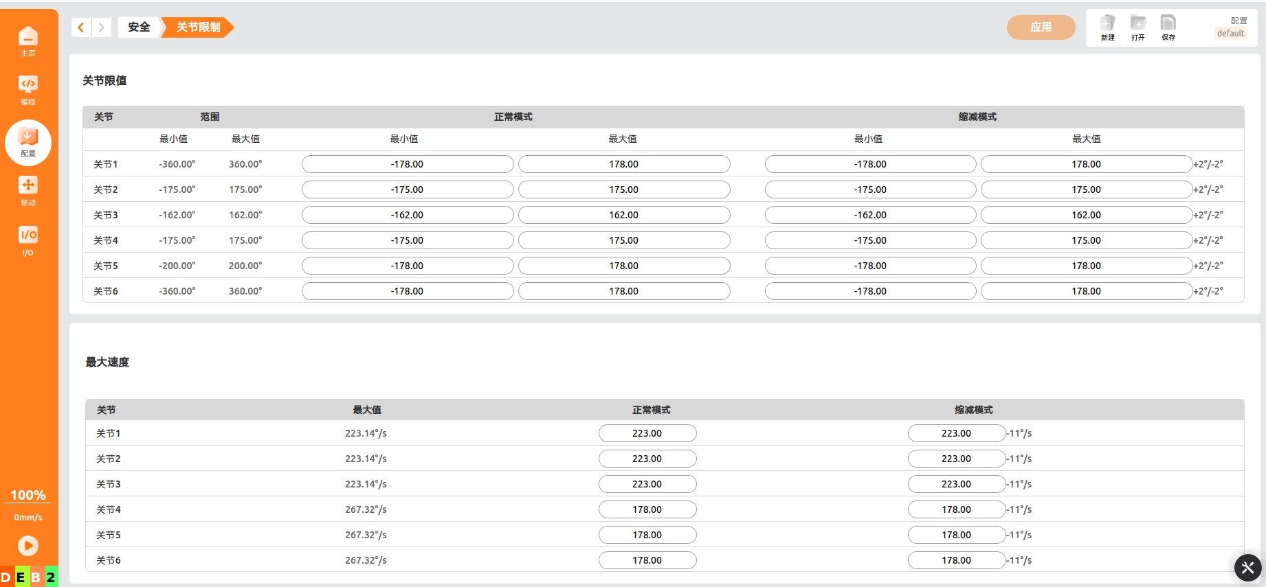Joint limit description: The 【Joint Limits】 interface sets the maximum limits that each robot arm joint can reach, restricting each joint's movement in joint space. You can set the rotation angle and maximum joint speed limit of each joint under 【Normal Mode】 or 【Reduced Mode】. • Values in 【Reduced Mode】 cannot be greater than those in 【Normal Mode】; otherwise the system prompts that they cannot be saved • The default values of joint maximum, joint minimum, and joint maximum speed limit are the maximum range; the user can only modify them within the default range

3.2 System Settings

3.2.1 Language Settings Feature Comparison

Feature	PE	ARCS
Language settings	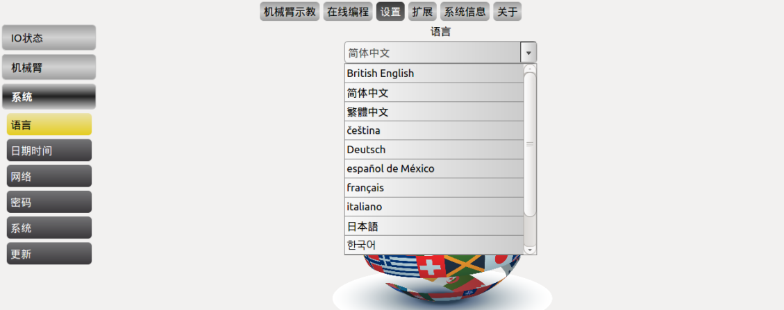Supported languages: Provides settings for English, Chinese (Simplified & Traditional), Czech, German, French, Italian, Japanese, and Korean.	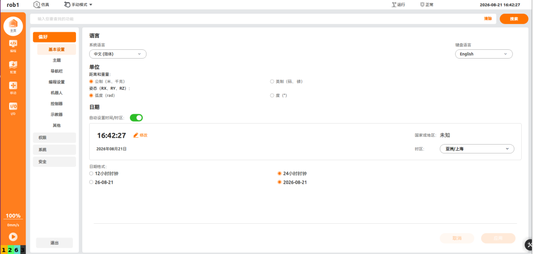System language: Supports Czech, English, Japanese, Korean, Russian, Simplified Chinese, and Traditional Chinese Keyboard language: Supports Chinese and English

3.2.2 Date and Time Settings Feature Comparison

Feature	PE	ARCS
Date and time settings	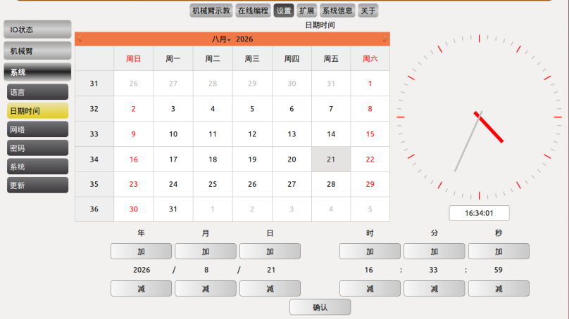Time settings: You can set the system date and time. Basic settings: You can set language, units, date, etc.	Unit: sets the system's units Date: sets the time and date format Time: supports two modes — follow the system time and custom time • Follow system time: automatically synchronized • Do not follow: click 【Modify】 to customize the time Apply: apply the settings Cancel: cancel the settings

3.2.3 Network Settings Feature Comparison

Feature	PE	ARCS
Network settings	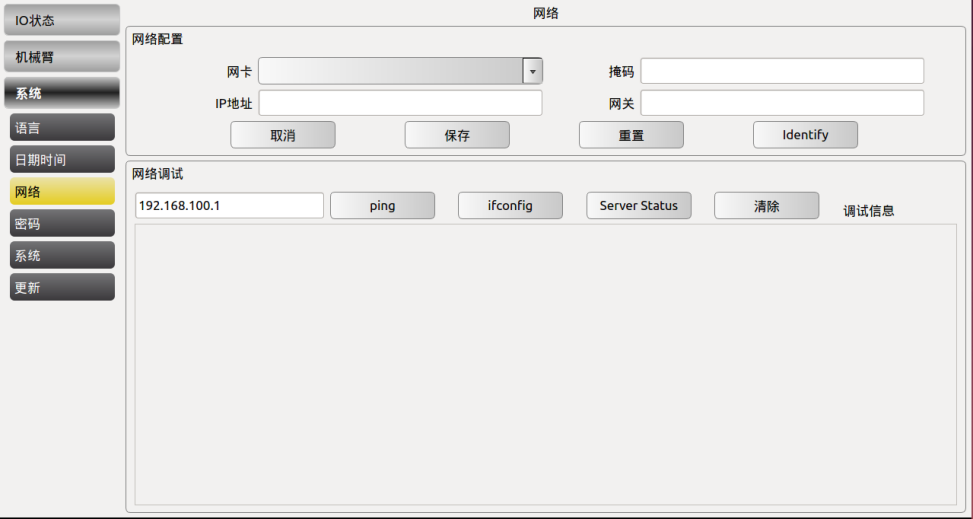Function description: The network settings unit is used for the network settings of third-party interface control. This interface configures the specified NIC name and its IP address, subnet mask, and default gateway. The network IP address of the third-party interface must be in the same network segment as the local machine's IP address. Network debugging: • ping: check whether the connection to the external device can be pinged • ifconfig: view NIC information • server status: check whether the robot arm server port is in the listening state	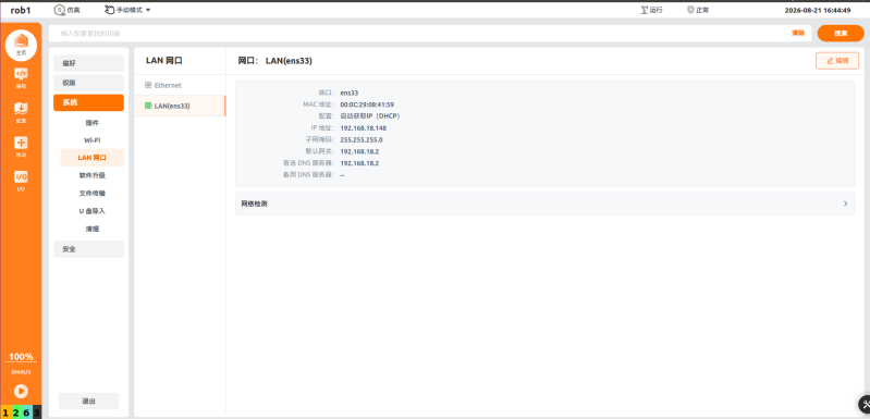Function description: 【Network】 configures the network for third-party interface control; after setting, the system can connect to an external network or a LAN. Notes: • The network IP address of the third-party interface must be in the same network segment as the local machine's IP address • Modifying the network configuration will interrupt the network connection. Please modify the configuration when the robot is idle, and ensure that programs and configurations are saved to avoid data loss • Please prefer using DHCP to connect to the network. If you choose the static-address mode, remember the IP address you set and ensure that it is free; otherwise the controller may not be reachable

3.2.4 Password Settings Feature Comparison

Feature	PE	ARCS
Password settings	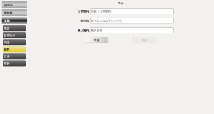Permission management: Provides two-level permission management with an administrator password and an operator password.	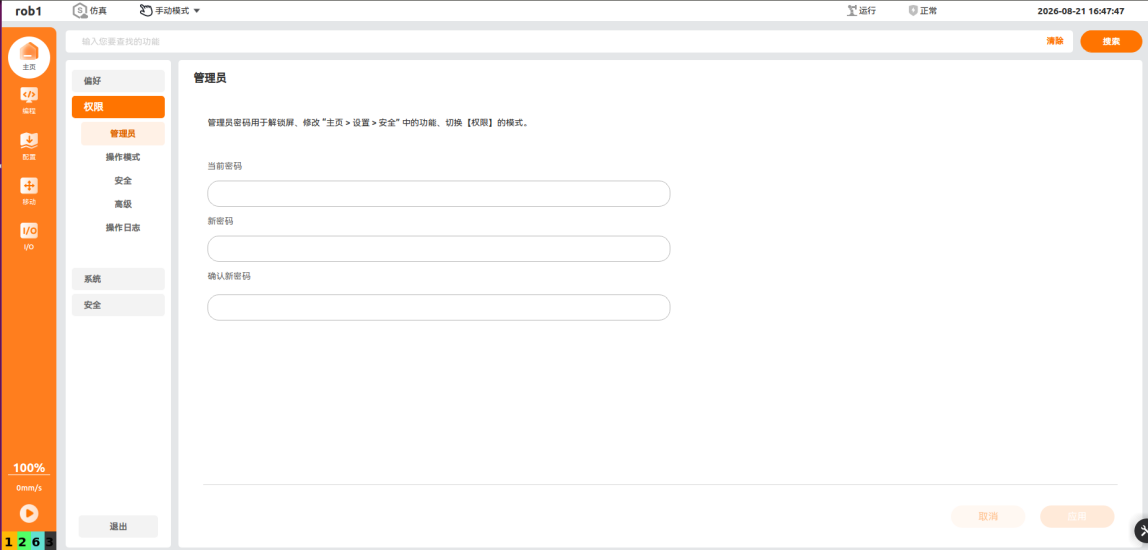Permission management: Provides setting and modification functions for three passwords — administrator, operating mode, and safety. Different passwords manage permissions for different functions.

3.2.5 Update Feature Comparison

Feature	PE	ARCS
Restore factory settings		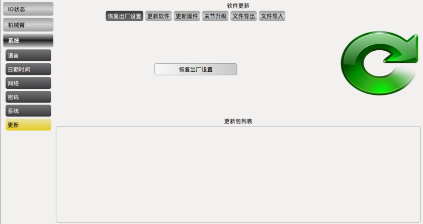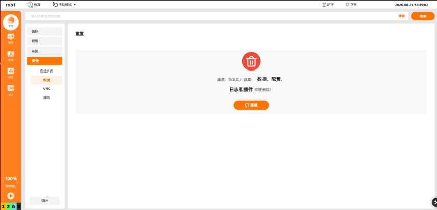The 【Restore】 interface can restore the system to factory settings.
Software/firmware update	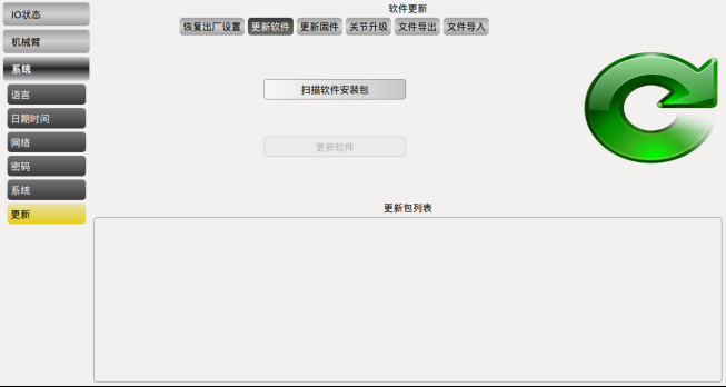Corresponding content software upgrade interface	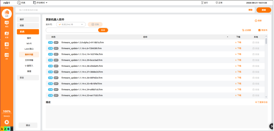AuboStudio supports both online and offline software updates. Online software update: The controller must be able to connect to the external network; download the installation package via 【Software Upgrade】 and install it. It supports switching to the current version and restarting to take effect. Offline software update: Download the installation package (.run file) from the official website and import it into the controller, then filter the local installation package via 【Software Upgrade】 to install it. Software version switch: Select the version from the drop-down menu to switch; it takes effect after restarting the controller.
Project file log export and import	Log export: You can click the 【Download】 button in the 【Home > Log】 card to export logs.	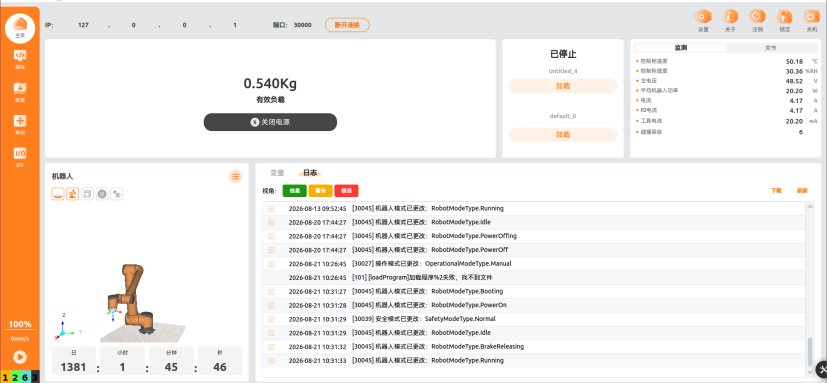Log export methods: • Local: save locally • USB drive: save to an external USB drive • LANDrop: transfer files via third-party software USB drive import: 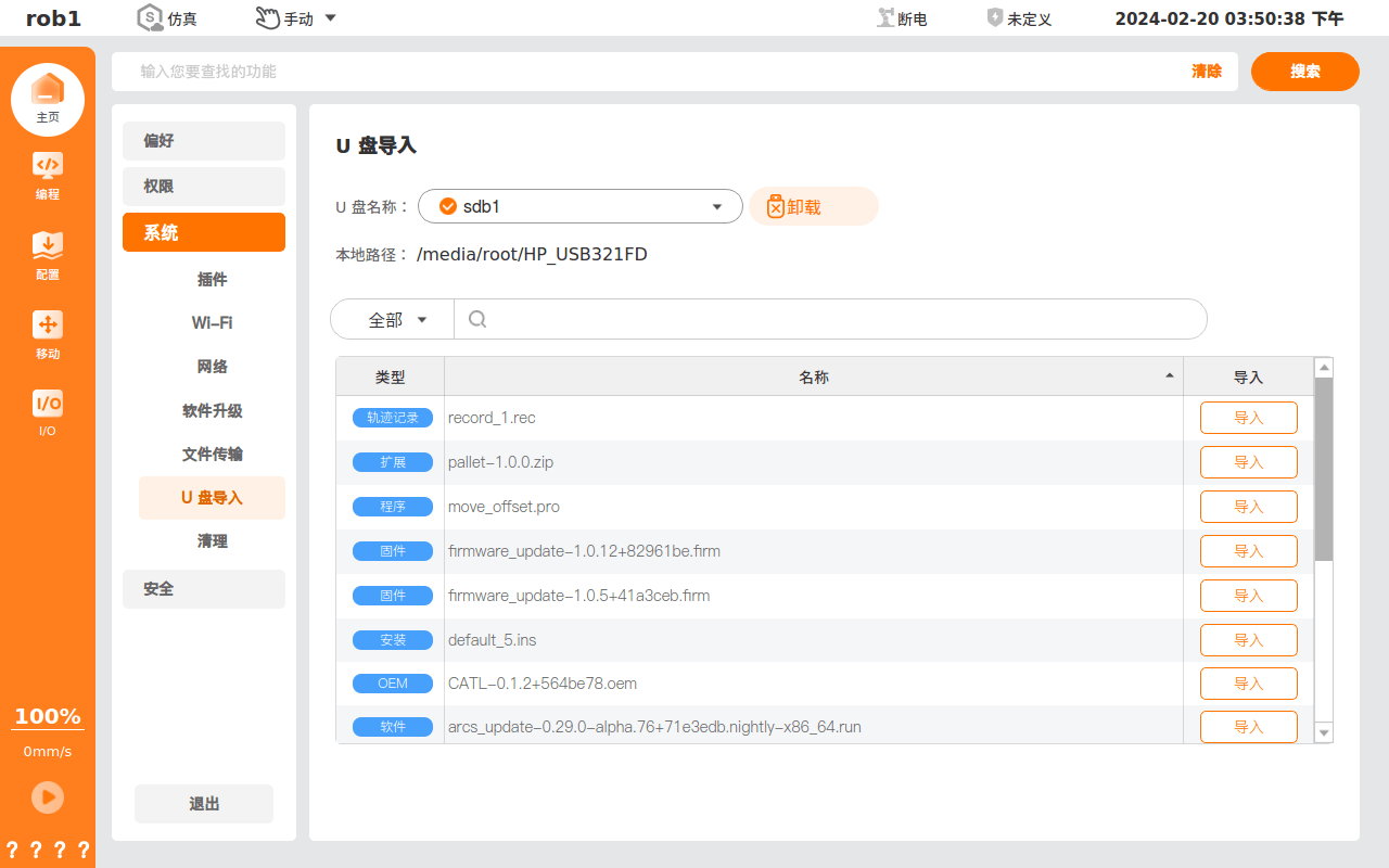After inserting the USB drive, the system recognizes it automatically; after mounting succeeds, files can be imported to the controller. Imported project files, installation configuration files, and installation packages are used under their corresponding function modules. After the operation is complete, unmount the USB drive before removing it.